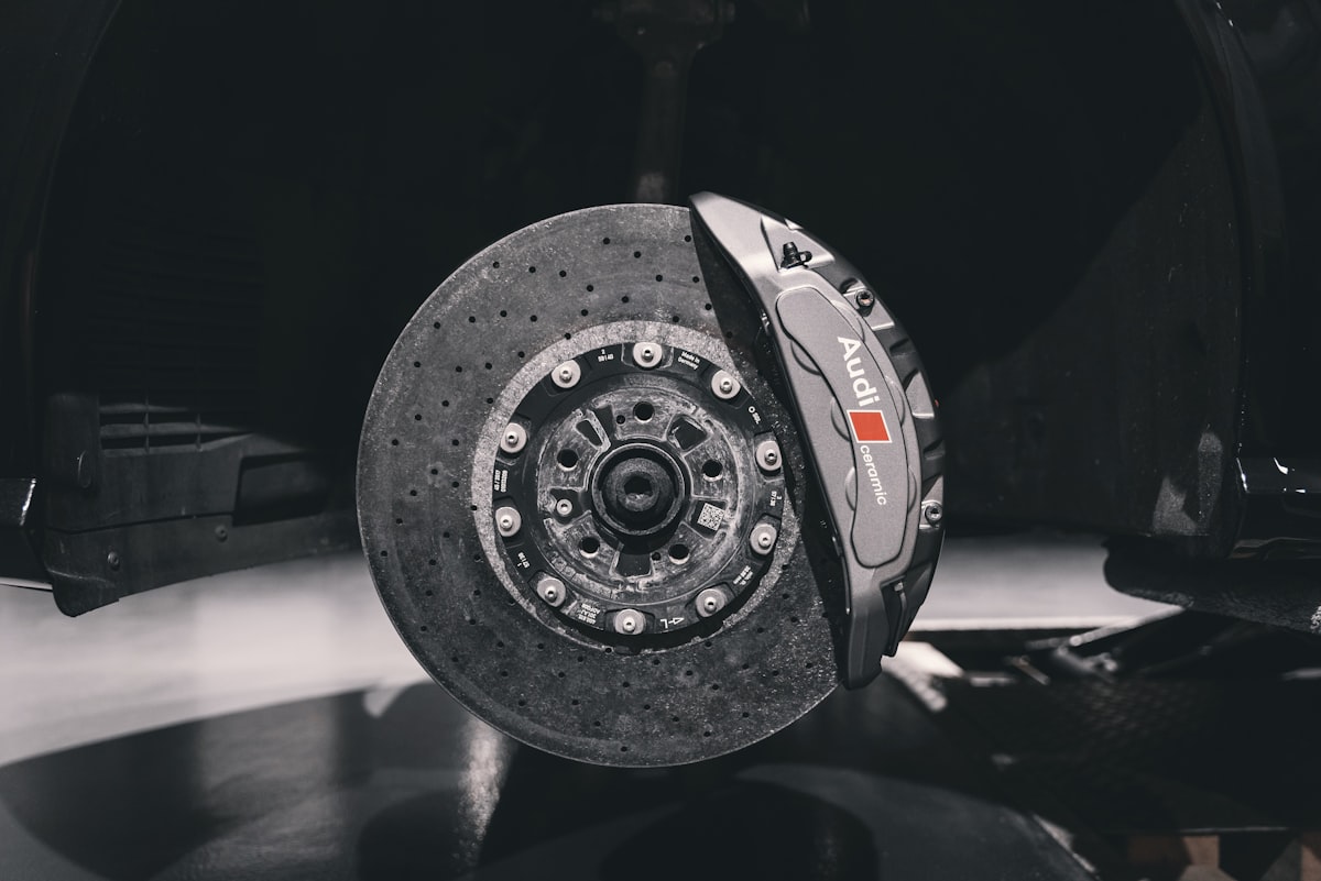
Estimating the working temperature of a brake disc
I used a lumped-body approach to approximate the properties of a brake disc and simulated its temperature increase after 100 braking maneuvers.

Modeling the temperature rise of a brake disk during a race without running a full-fledged thermal transfer FEA
Did you know that you can estimate the temperature trend of a brake disc using an iterative script in MATLAB or Python?
I used a lumped-body approach to approximate the properties of an FSAE brake disc and simulated its temperature increase after 100 braking maneuvers. Let me show you how I did it.
Why brake discs get hot
The braking system of any vehicle converts kinetic energy into thermal energy through the friction between the brake pads and rotors. During a braking maneuver on a level surface, the amount of energy that the brakes system dissipates is given by
\[\Delta E_b = \frac{m}{2} ({V_1}^2 - {V_2}^2 ) + \frac{I}{2} ({\omega_1}^2- {\omega_2}^2) - F_{drag} d_{brake}\]
where m is the vehicle mass, I is the mass moment of inertia of the rotating parts. V is the vehicle speed and ω is the angular speed of the wheels.
The subscripts 1 and 2 refer to the conditions before and after braking, respectively. The last term is the aerodynamic drag energy over the distance covered while braking.
Part of this energy is transferred to the brakes in the form of heat, so the temperature of the rotors and calipers is increased.
Here I'm not considering the rolling resistance of the car, so this is an overly conservative estimate of how much energy needs to be dissipated by the brakes.
For a brake disc, the temperature rise during a braking maneuver is given in a simplified way by
\[ \Delta T = \frac{E_{b_{i}} \cdot p}{m_{disc} \cdot C_p}\]
where Ebi is the portion of the total energy dissipated by a single disc in the axle i. The mass of the brake disc is m_disc, and Cp is the specific heat of the material it is made of. The factor p determines the proportion of the total heat that is transferred to the rotor.
This heat partition coefficient p can be computed as:
\[ p=\frac{\sqrt{k_{disc} C_{p_{disc}} \rho_{disc} } S_{disc}}{\sqrt{k_{disc} C_{p_{disc}} \rho_{disc} } S_{disc} + \sqrt{k_{pads} C_{p_{pads}} \rho_{pads} } S_{pads} } \]
and as you can see, it depends on the thermal conductivity k, specific heat Cp and density ρ of the materials in contact (brake disc and pads), and their surface areas.
For continuous braking situations, this heat partition coefficient can also be modeled in terms of the thermal resistance of the components involved
%Thermal resistance of the Brake rotor
Rd= 1/(A_total*h_conv_disc);

%Thermal resistance of the pad
Rp= 1/hp_conv+t_pad/(k_pad*S_p)+t_plate/(k_plate*S_p);

%Heat Partition Coefficient
p=1/(1+Rd/Rp);
This approach is more realistic since it involves the convection coefficient of the pad and the disc. However, knowing the value of those isn't a very simple task. I wrote another article about how I attempted to estimate the convection coefficient for the brake disc.
But how does the temperature change over time?
The braking power in a particular wheel can be considered equal to the amount of energy that is converted into heat divided by the duration of the braking maneuver:
\[P=\frac{d(E_{b_{i}} )}{dt} \]
For a constant brake torque applied to the rotor, the instantaneous power can be obtained from the product
\[P_{i_{(t)}} = T_{brake} \cdot \omega_{i_{(t)}} \]
Then, the temperature rise can be computed for different instants of time using
\[\Delta T = \frac{ ( T_{brake} \cdot \omega_{i{(t)}} \cdot p - \dot{Q}{conv_{i}} - \dot{Q}{rad_{i}} ) t{i} }{ m_{disc} \cdot C_{p_{disc}} } \]
As you can see, this equation also includes the heat losses per unit of time due to the convection and radiation heat transfer, respectively.
A lumped model
Considering a uniform temperature distribution within the disc, its temperature can be modeled as:
\[\frac{T- T_∞}{T_i - T_∞} = e^{-Bi \cdot Fo}\]
where T represents the rotor temperature at a given instant of time. The subscript i corresponds to the initial thermal conditions and ∞ refers to the temperature of the air surrounding the disc. Bi and Fo represent the Biot number and Fourier number, respectively.
The Biot number is a dimensionless parameter that indicates the proportion between the temperature gradient in a solid (the brake disc) and the temperature difference between its surface and the fluid around it (the air).
\[Bi=\frac{hL_c}{k} \]
The letter h represents the convection heat transfer coefficient, k is the thermal conductivity of the solid material.
If Bi ≪ 0.1, the conduction heat transfer problem is characterized by the Fourier number, which is a function of α (the thermal diffusivity) and time. It is given by:
\[Fo=\frac{\alpha t}{L_c^2 }\]
where L_c is the characteristic length of the rotor body, defined as the ratio between its total volume and surface area.
The thermal diffusivity, α gives you an idea of the rate at which heat is transferred from the hot end to the cold end of the material, and is given by
\[\alpha = \frac{k}{\rho \cdot C_p}\]
Implementing this in a MATLAB script
I wrote a code to simulate a fixed number of braking maneuvers, each one followed by a fixed amount of cooling time.
I calculated the temperature rise while braking and the amount of heat dissipated from convection and radiation to the surroundings of the disc - I neglected conduction to simplify the analysis.
The idea of doing this is to simulate the average braking maneuver performed in a particular circuit, to see the discs' temperature trend. This can be used, for example, to compare the impact of different parameters, like disc size, weight, and material.
Here is an example (pseudocode).
tcool = 5; % sec
V_start = 70; % km/h
V_final = 45; % km/h
n = 100; % number of braking maneuvers to simulate
T_disc_start = 60 + 273; % K
P_avg; % Average power transferred to the disc during a braking maneuver

for i = 1:2*n

  if i == 1
    T_disc(i) = T_disc_start;

  else if i > 1 && mod(i,2) == 0  % even numbers are used for cooling
    T_disc(i) = T_disc(i-1) + Dt;

  else % odd numbers are for braking

      BixFo=h_conv*A_total*tcool/(rho_metal*V_disc*Cp_metal);

      % The temperature is increased with an exponentially smaller effect
      % with every new braking maneuver
      T_disc(i)=T_air+(1-exp(-i*BixFo))*DT_f/(1-exp(-BixFo));
  end

    % Compute H_convection
    H_convection=(h_conv(i)*A_disc)*(T_disc(i)-T_air);

    % Compute H_radiation
    H_radiation= 5.670367*10^-8*A_disc*2*(T_disc(i)-T_air)^4;

    Dt_cool = (H_convection + H_radiation)*tcool / (rho_metal* V_disc * Cp_metal);

    % During braking, only a portion of the disc's surface is used for cooling
    f = (S_d - (2*S_p)) / S_d; % ~ 0.8
    Dt_brake = P_avg * t_stop * p / (rho_metal* V_disc * Cp_metal);
    Dt = Dt_brake + Dt_cool * f;
endAnd here is the result (I ran this for different material properties).
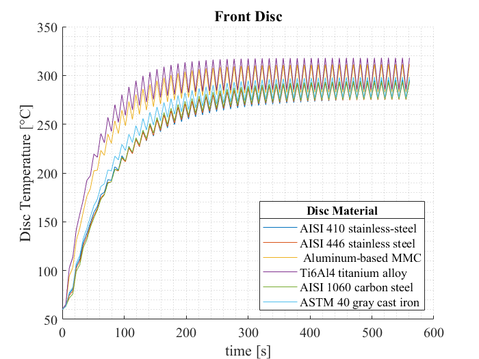
There's room for improvement here
As you can see the results basically show a sequence of straight lines. One with positive slope (braking, thus, heating) followed by another one with negative slope (cooling).
This is a heavy simplification of how the temperature changes over time, but it's close enough if we want to get a trend and average values.
To make an even more realistic simulation, braking maneuvers of different intensities could be used as input, computing the braking power and cooling for each one of them. This way it would be a more realistic representation of an actual circuit.
From the programming point of view, using a for loop with if-else statements is not the most elegant or efficient way of doing this - it is, however the easiest one to understand if you are not familiar with array operations.
A better way would be creating a function to calculate the power losses, and an input array containing the speeds at the start and end of each braking maneuver.
The input array could be passed as an argument to the function, to return an array of the temperatures.
Indexing operations can be used to perform different operations on the rows of the array, eliminating the for loop altogether. I've done that before on MATLAB and Python.
Now let's talk a bit more about the boundary conditions.
How did I choose which braking maneuver to replicate?
I'm glad you asked.
I had access to CAN data logs from previous races of a similar race car, so I analyzed them to determine a representative value of the average braking.
It was similar to what I did when showing an example of using Matlab and statistics to analyze vehicle data.
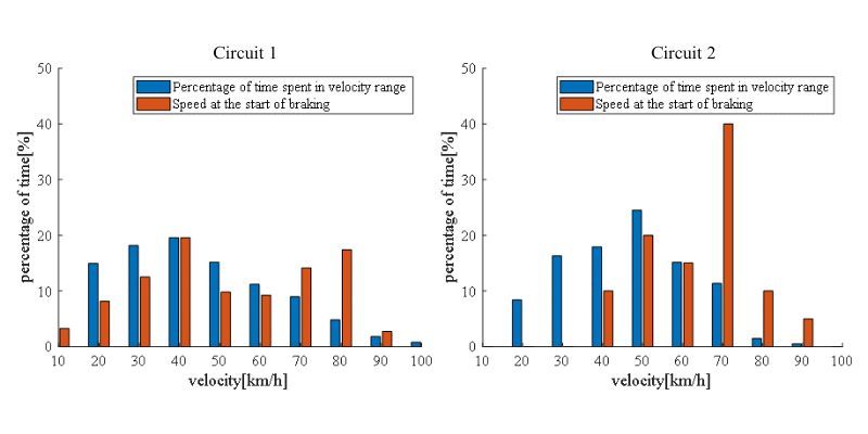
Clearly, the conditions at which the braking maneuvers take place are very different for each circuit and vary from driver to driver. Nevertheless, the analysis showed that the most common speed range at which the drivers started to brake for circuit 2 was between 50 and 70 km/h.
What about the convection coefficient?
That's for another post. However, if you are interested, you can have a look at the live script that I published on this Github repo, showing how I computed an approximate value of the heat exchange coefficient.
How accurate are the results?
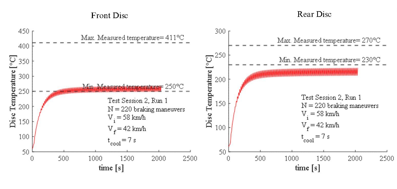
Unfortunately, I never got the chance to record the actual temperatures of the discs during exercise - that is, real temperature measurements while the car was running.
I could only use a Fluke Ti110 thermal camera to register the temperatures immediately after some full stops planned during and at the end of each run, so this is only indicative data.
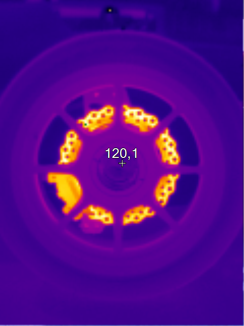
When comparing the predictions made with this approach and the measurements obtained from the thermal camera, we can see that the analytic calculation underestimates the actual temperatures.
Well, certainly you can't expect superb accuracy with this simplified approach. However, I do think that if you find and "tune" the input parameters needed for an actual car, you'd be able to get a relatively good estimate of the average working temperature of the brakes.
Of course, this can be adjusted by changing the inputs provided to the simulation. Especially the boundary conditions. For example, the real start and end speeds might be different, and the time allowed for cooling could be shorter, as well as the convection coefficient of the brake disc.
The only way to find out how accurate is this estimated average temperature would be to record the actual temperatures of the brakes during exercise.
For sure, peak values cannot be captured with this approach, and this is in no way a method that can be used to design the thermomechanical properties of a brake disc.
Also, it's important to remember that this is just a tool for early design stages, and can only be used if properly "tuned" based on data already available.
If you are interested, read my other posts about this topic:
References:
|
[1] |
R. Limpert, Brake Design and Safety, Warrendale, PA.: Society of
Automotive Engineers, Inc., 1999. |
|
[2] |
F. P. Incropera, D. P. Dewitt, T. L. Bergman and A. S. Lavine,
Fundamentals of Heat and Mass Transfer, 6th Edition, John Wiley & Sons,
Inc., 2007. |
|
[3] |
A. Day, Braking of Road Vehicles, Elsevier Inc., 2014. |