Brake system load distribution study - MATLAB approach

When I was part of the Formula Student team of Politecnico di Torino, I was working on sizing the braking system of a race car.

As an Automotive Engineering student, I already knew the concepts of vehicle dynamics and brake systems. Still, the books won't give you an actual recipe for applying those to a real system.

How do you choose the dimensions for the brake calipers and pistons for an FSAE car? Well, there's a lot to consider for this, which includes basic geometric constraints (how much space is available?) and weight limits (is there an unsprung mass design target?),  and of course, the target deceleration that the car needs to achieve.

On top of this, there's also the need to have a "balanced" distribution of the braking forces. This is the so-called brake load repartition, which basically answers the question

"How much braking force will be available on the rear axle, when applying this much braking force on the front one?"

This is not so easy to compute with a simple force balance. As you might have guessed.

The whole thing is an iterative process you wouldn't ever want to solve by hand.

On one hand, you have the relationship between the force applied to the brake pedal, and the brake torque applied on the front and rear wheels.

On the other hand, the amount of braking force applied on the front axle also depends on how much friction is available at the tire contact patch and how much load is being transferred longitudinally due to the deceleration of the vehicle and aero forces.

To solve this, you'd need a full-on vehicle simulation. But you can study the behavior of the system using some coding. Let me show you how I did it.

Imagine you have a given set of hydraulic properties of the brakes and overall vehicle characteristics. Piston diameters for calipers and master cylinders, rotor diameters, wheel radius, wheelbase, height of the center of gravity, estimated aero loads...

%% Vehicle data
rho_air=1.16; %kg/m3
front_area=1; %m2
Cz_frontxS=1.504;
Cz_rearxS=1.696;
CxS=1.12;
m=275; %kg
g=9.81; %m/s^2
l= 1.525; a=0.808; b=l-a; hcg=0.245; %m
 
%% Brake system parameters
%This section contains all the functional parameters of the brake system.
%The parameter values can be modified to evaluate different configurations.

%Pedal Box
Pedal_ratio=3.03 %Brake pedal mechanical advantage
Preload=0; %Spring preload [N]
fMC_Diam=19 %Front master cylinder piston diameter[mm] 
rMC_Diam=16 %Rear master cylinder piston diameter[mm]
AMCf=pi*fMC_Diam^2/4 % Section area of front MC mm^2
AMCr=pi*rMC_Diam^2/4 % Section area of rear MC mm^2


%Brake Calipers
fCaliper_diam=24 %Front calipers piston diameter[mm]
fCaliper_PistonQty=4
ACf=pi*fCaliper_diam^2/4*fCaliper_PistonQty % Front caliper pistons area mm^2
rCaliper_diam=24 %Rear calipers piston diameter[mm]
rCaliper_PistonQty=2
ACr=pi*rCaliper_diam^2/4*rCaliper_PistonQty % Rear caliper pistons area mm^2 

frpad=94 %front caliper effective radius
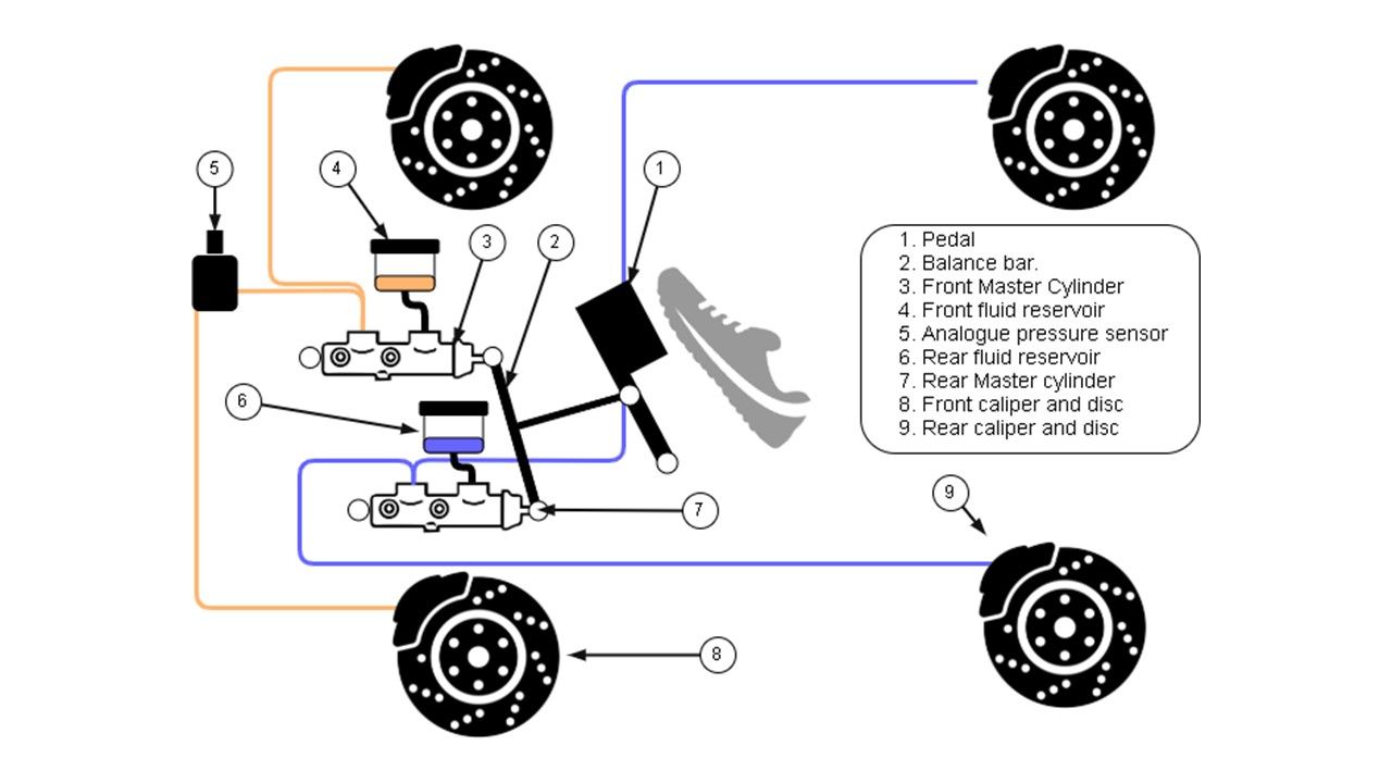
rrpad=83 %Rear caliper effective radius

The brake repartition starts from knowing how the pedal force is distributed between the front and rear hydraulic circuits. For a given value of pedal force, this ratio is given by:

\[𝐾_𝑏 = \frac{𝑇_{brake_1}}{𝑇_{brake_2}} = \frac{\frac{𝐹_{pedal}}{A_{MC_1}}\times\frac{l_2}{L_{bar}} \times r_{pad_1} \times {A_{C_1}} \times \mu_{pad_i}}{\frac{𝐹_{pedal}}{A_{MC_2}}\times\frac{l_1}{L_{bar}} \times r_{pad_2} \times {A_{C_2}} \times \mu_{pad_i}}\]

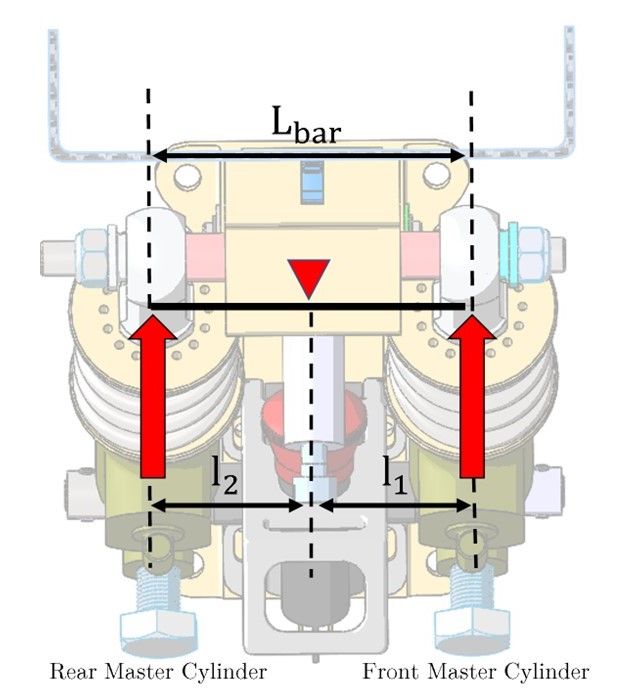
Having defined the characteristics of the brake calipers, master cylinders, and brake discs, the only variable that can be used to adjust the proportion of force being applied to the front circuit is the balance bar position, which gives the front bias ratio:

\[ \%Front \space Bias \space = \frac{l_2}{L_{bar}} \times 100\]

And the force in the rear axle will be:

\[F_{x_{2_{real}}} = \frac{F_{x_{1_{input}}}}{K_b} \]

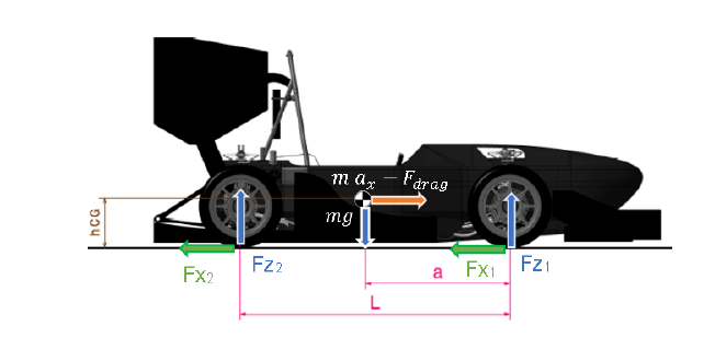
Instead, to know the ideal force distribution, you need to solve

\[F_{x_{1_{input}}} - F_{x_{2_{ideal}}} = \mu_x (\frac{ m g}{l} (b-a + \mu_x 2 h_{cg}) + A - B + C) \]

where

\[A = (F_{z_{aero_1}} - F_{z_{aero_2}})\]
\[B = \frac{2 F_{drag} h_{cg}}{l}\]
\[C = \frac{2 \mu_x (F_{z_{aero_1}} + F_{z_{aero_2}}) h_{cg}}{l}\]
\[\mu_x = \frac{F_{x_{1_{input}}} + F_{x_{2_{ideal}}}}{mg + F_{z_{aero_1}} + F_{z_{aero_2}}}\]

Solving this equation is not difficult. It is simply very tedious.

This is where scripting comes in.

Python and Matlab are great for solving this kind of problem. In this case, I used Matlab, since I had access to a full Academic license, being enrolled as a MSc. student at Politecnico di Torino.

The idea of making a script is to make it do the heavy lifting for us

In this case, I used symbolic computing to define the variables and have Matlab solve the equations for me.

First, I verified that the results were correct, looking at the solution with symbolic variables only.

%% Define symbols
syms Fx1 Fx2 b a l hcg m g Fzaerof Fzaeror mux F_drag;

%Ideal braking equations
(Fx1-Fx2) == mux*(m*g/l*(b-a+mux*2*hcg) + ...
					(Fzaerof-Fzaeror) - ...
                    2*F_drag*hcg/l + ...
                    2*mux*(Fzaerof+Fzaeror)*hcg/l)

mux = (Fx1+Fx2) / (m*g+Fzaerof+Fzaeror)


eqn = mux*(m*g/l*(b-a+mux*2*hcg) + ...
			(Fzaerof-Fzaeror) - ...
            2*F_drag*hcg/l + ...
            2*mux*(Fzaerof+Fzaeror)*hcg/l) - (Fx1-Fx2)

%Solve for the force in the rear axle
solve(eqn,Fx2)

Next, I made a script to compute the results over a range of input front brake forces, and also at varying vehicle speeds.

To do this, I created a vector with speed values linearly spaced from 40 km/h up to 110 km/h. So I would compute the load repartition when braking from each one of those speeds.

Calculating the brake load distribution

To iterate through different front axle force values, I computed the maximum force at the front axle during a hard braking maneuver. The result was 4500 N, so I decided to iterate over 45 steps, from 0 to 4500 N, with 100 N increments.

This was simply a for loop, within another for loop.

The "outer" loop iterates over the vehicle speeds. The inner loop evaluates the equation for the force at the rear axle, for all values of force at the front one.

%% Solve the symbolic equations for different values of initial speed
% Maximum load on front axle at max. deceleration was calculated at 4500 N
% So we choose to compute the load distribution for 45 increments of 100 N 
n_steps = 45;
f_step = 100;

j=1;
% Create vehicle speed vector. Assumes speed decreases linearly
v=linspace(40/3.6,110/3.6,8);

% Loop through speed values
for V= v
    
    % Evaluate aero forces at the current speed
    F_drag(j) = 0.5*rho_air*front_area*CxS*V^2; %[N]
    Fz_aero_front = 0.5*rho_air*front_area*Cz_frontxS*V^2; %[N]
    Fz_aero_rear = 0.5*rho_air*front_area*Cz_rearxS*V^2; 
    Fzaerof = Fz_aero_front; Fzaeror=Fz_aero_rear;
    
    % Define mux with the current values of aero forces
    syms Fx1 Fx2
    mux = (Fx1+Fx2)/(m*g+Fzaerof+Fzaeror);
    
    eqn = mux*(m*g/l*(b-a+mux*2*hcg) + ...
    	      (Fzaerof-Fzaeror) - ...
              2*F_drag(j)*hcg/l + ...
              2*mux*(Fzaerof+Fzaeror)*hcg/l) - (Fx1-Fx2);
    
    Fx1_it=0;
    
        for i=1:n_steps  
        Fx1=Fx1_it;
        RATIO=subs(eqn);
        SolFx2=solve(RATIO,Fx2,'real',true); %'ReturnConditions',true
        Fx2_calc(i)=double(SolFx2(2));
        g_decel(j,i)=(Fx1_it+Fx2_calc(i)-F_drag(j))/(m*g);
        
        % Increment force at front axis for next iteration
        Fx1_it=Fx1_it + f_step;
        end

 FX2(j,:)=Fx2_calc;
 j=j+1;

end

Fx1_input=linspace(0,Fx1_it,n);
[numRows,numCols] = size(FX2);

This allowed me to evaluate whether the behavior of the braking system was compatible with the ideal load repartition of the car, over the complete range of longitudinal force for the front and rear axles.

The figure below illustrates the results.

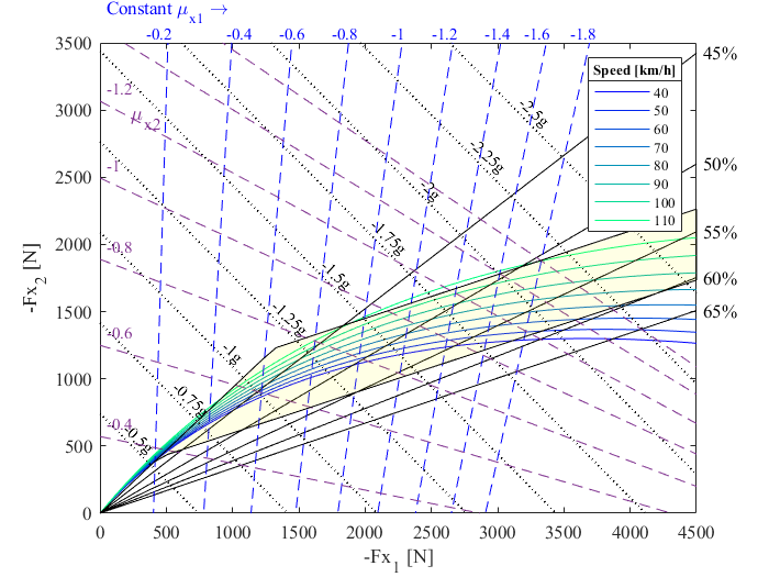
The parabolas show the ideal repartition of the forces between the front and rear axles when braking from different vehicle speeds. They are a function of the geometry and inertia of the car, regardless of the configuration of the braking system.

The straight, black lines represent the response of the system, for different settings of the balance bar (Front Bias %). To compute those, I used another for loop:

bar_ratio=linspace(0.45/0.55,0.65/0.35,5)
front_bias=linspace(0.45,0.65,length(bar_ratio))
    for k=1:length(bar_ratio)
        Tqratio=bar_ratio(k)*(AMCr*frpad*ACf)/(AMCf*rrpad*ACr);
        Fx2_real=Fx1_input/Tqratio;
    end

The critical deceleration of the car is the theoretical maximum rate at which it can be braked while maintaining directional stability. It is given by the interception between an ideal force distribution line and a system response line.

In this case, for instance, for a 50% front bias, the car would theoretically be able to brake at a maximum of ~1.6 g.

This is, of course, valid only under ideal conditions, but can be used as a reference when making changes to the design.

The full script I used when making this analysis is available on my GitHub repository and I also published it on MathWorks File Exchange.

Conclusion

This approach to studying the load distribution of a car is a basic exercise, and I think it’s taught in most Automotive Engineering courses. It is, however, a useful tool for understanding how the system behaves in different conditions, especially during early design stages.

I hope this is useful for people who are curious about vehicle dynamics, or younger students starting a Formula SAE or Formula Student team.

Besides the domain knowledge about the braking system, another message I’d like to pass on is how making simple scripts is a huge tool for any engineer, even if you are not a software developer.

As an Engineer, your knowledge of how the physics of a particular system work is more valuable than solving the equations behind them over and over again, especially if there are going to be design changes.

Here, I solved simple but tedious equations several times and evaluated the performance of a system over its operating range.

If you learn to create quick scripts like this, you'll be able to leverage computing power for doing much more complex tasks. This will open up new possibilities for you to go further when designing or analyzing components or systems.

If you are interested in learning more, I'm sharing examples of simple engineering computations with MATLAB and Python. It's a section of my blog that I'm calling Engineering scripts.

Subscribe to my newsletter to stay up to date with my new articles!