Using MATLAB and statistics to analyze raw vehicle data

It’s been a couple of weeks since I published the initial post of a series about replacing MATLAB with Python. If you haven’t read it yet, the short story is that I forced myself to use Python to do some of the tasks I would normally do using MATLAB at work. I committed to sharing what I've learned in the process, including simple code examples to illustrate it, which may be useful if you are interested in doing something similar. I'm no expert, though, so don't expect to see super complex codes or analyses here!

However, I figured that it would be easier to share separately the MATLAB examples and the Python ones. Mainly because, otherwise, the articles would be excessively long.

In this second entry, I am sharing an example of the workflow I would follow for getting insights from real-world data using histograms and some very basic statistics.

We will be using two datasets containing raw data logged from the CAN bus of a Formula Student Electric car. The data is already stored in a .CSV format to make this more “universal”, since there are different formats for storing automotive data.

RaceCar data - Google Drive

Google Drive

For context, the datasets were recorded while two drivers tested exactly the same vehicle in exactly the same circuit. On the same day, a few minutes apart from each other. There was no transponder installed for recording the lap time accurately, and the information from the electric motors is not available for some reason. This is about all the context we need. We want to analyze the data from both drivers but won’t go into the details.

Let’s jump right into it!

When using MATLAB, I load the data from the CSV files, store the data in some variables, and define the constants that I am going to use later.

%% Get descriptive statistics from CAN datalogs
close all, clc

filename1 = 'driver1.csv';
filename2 = 'driver2.csv';

% Read file 1
t1 = readtable(filename1);
% Verify that I get all the columns I need
t1.Properties.VariableNames

% Repeat for file 2
t2 = readtable(filename2);
t2.Properties.VariableNames

%% Define vehicle parameters
% This was a Formula Student Electric car, with four in-wheel electric
% motors coupled to an epicyclic transmission, all four with the same gear ratio
gear_ratio = 16;    % Transmission gear ratio
r = 0.263;          % Wheel radius [m]

I'm using tables to handle the data because I find them very easy to use. Additionally, using tables in MATLAB can help you transition more easily to using Pandas data frames if you want to. This will be more evident later on. Tables are not the most efficient way to handle very large datasets, but they do offer some convenience and if you know how to index them, they work great.

Let’s move on. I have the data loaded on MATLAB, so now I can do stuff. As I’ve mentioned before, a good practice is to start with a simple plot or, in this case, a bunch of them, since we have few variables and files.

%% Plot the data available, just to have a quick overview
figure('Position', [10 10 1200 400])
tiledlayout('flow', 'TileSpacing', 'compact')

for i_plot = 2:size(t1,2)
    
    nexttile
    plot(t1.Time_s, t1{:, i_plot}, 'DisplayName', '1')
    hold on
    plot(t2.Time_s, t2{:, i_plot}, 'DisplayName', '2')
    title(t1.Properties.VariableNames{i_plot}, 'Interpreter' , 'none')
    legend
    
end

Great! we have comparable data in both files. We have pressure data from a sensor in the hydraulic circuit of the car, raw acceleration data from an IMU, and the rotational speed of the four motors attached to the wheels. There is a slight time offset between the two data sets, and one of them is a bit longer. This is raw data, so it is something completely normal.

Let’s find out which driver was faster. To do this, we need to compute the vehicle speed.

Estimating the vehicle speeds

This is not easy at all - it might seem, but it is not - at least if you want to do it accurately. What we can do is settle for a simplified calculation assuming the following:

• When the vehicle is accelerating, the speed of the car is similar to the speed of the contact point of the slowest tire, i.e. the one that rotates slower than the others and thus has a smaller slip ratio.
• On the other hand, when the car is braking, the slowest tire is most likely locked, with a higher absolute slip ratio than the others. So in this case the vehicle's speed is closer to that of the fastest spinning tire - no accelerating torque is present.

This is a rough estimate but should be enough for this analysis. But before we do this, we need to do some work to clean up the raw acceleration data. I will remove the DC offset, and filter the noise.

%% Filter the longitudinal acceleration

% Compute the sum of the wheel speeds
sum_of_speeds1 = t1.spd_rpmFR + t1.spd_rpmFL + t1.spd_rpmRR + t1.spd_rpmRL;
sum_of_speeds2 = t2.spd_rpmFR + t2.spd_rpmFL + t2.spd_rpmRR + t2.spd_rpmRL;

% Remove any DC - offset from the raw acceleration data
t1.AccXNoOffs = t1.AccX - median(table2array(t1(sum_of_speeds1 == 0, 'AccX')));
t2.AccXNoOffs = t2.AccX - median(table2array(t2(sum_of_speeds2 == 0, 'AccX')));

% Filter the signals
t1.AccX = sgolayfilt(t1.AccXNoOffs, 3, 101);
t2.AccX = sgolayfilt(t2.AccXNoOffs, 3, 101);

% COmpare the signals
figure('Position', [10 10 1200 400]);
hold on
plot(t1.Time_s, t1.AccXNoOffs, '-k', 'DisplayName', 'Raw AccX (removed DC offset)', 'linewidth', .5)
plot(t1.Time_s, t1.AccX, '-r', 'DisplayName', 'AccX (filtered)', 'linewidth', 1.5 )
xlim([600, 650])
xlabel('Time [seconds]')
ylabel("Acceleration [G - units]")
legend
grid minor

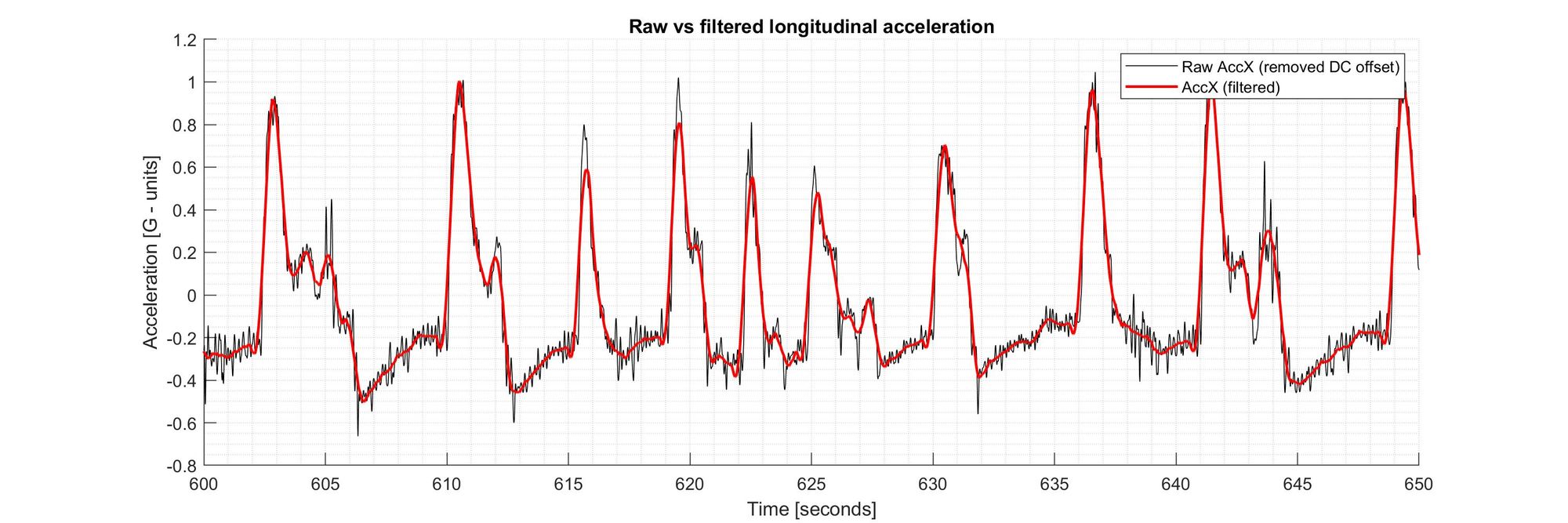
I filtered the acceleration signals using a Finite-Impulse-Response filter, in this case, a Savitzky–Golay filter. This type of filter does a good job preserving the height and location of the peaks and the area below them. Implementing this type of filter in MATLAB is as simple as just typing the sgolay command and including some parameters chosen accordingly. But only if you have the Signal Processing Toolbox license. So this might be one of the reasons to consider using free software options. Of course, with a little more work, you can implement a similar filter yourself using “standard” MATLAB commands. (edit: if you actually check the book Introduction to Signal Processing cited in the MATLAB documentation of the filter, you can actually see the implementation for many types of digital filters both in MATLAB and C, and download the files. Cool!)

Now, how to determine the vehicle speed using the approach I mentioned before?

Easy, right? Just make a for loop and iterate through the rows of the table. When the acceleration is positive take the minimum wheel speed, when it is negative, take the maximum one. And of course, convert each value to linear speed.

%% Estimate the vehicle speed: the for-loop way
% Extract the wheel rotational speed data from the two files
wRPM1 = t1(:,{'spd_rpmFL', 'spd_rpmFR', 'spd_rpmRL', 'spd_rpmRR'}); 
wRPM2 = t2(:,{'spd_rpmFL', 'spd_rpmFR', 'spd_rpmRL', 'spd_rpmRR'});

tic
for i_ax1=1:height(wRPM1)
    
   if t1.AccX(i_ax1,1)>0
       VEL1_for(i_ax1,1)=min(wRPM1{i_ax1,:})*(pi/30)*r/gear_ratio*3.6;
   else
       VEL1_for(i_ax1,1)=max(wRPM1{i_ax1,:})*(pi/30)*r/gear_ratio*3.6;
   end
end
toc % Elapsed time is 289.592689 seconds. <--- NOT GOOD!

That took forever! I don't want to wait that much time when doing this kind of thing! What if the data grows larger, or if I need to compare 100 files instead of 2, should I wait 4 hours? Maybe my PC is not the fastest, but there has to be a better way!

Fortunately, yes, there is a better way. We can use indexing methods instead of for loops.

%% Estimate the vehicle speed: Release the power of table indexing
tic

% Create empty columns for storing the vehicle speed
t1.Veh_Spd = zeros(height(t1), 1);
t2.Veh_Spd = zeros(height(t2), 1);

t1(t1.AccX > 0, 'Veh_Spd') = table(min(t1{t1.AccX > 0,...
    {'spd_rpmFL','spd_rpmFR','spd_rpmRL','spd_rpmRR'}}, [], 2)*pi/30*r/gear_ratio*3.6);
t1(t1.AccX <= 0, 'Veh_Spd') = table(max(t1{t1.AccX <= 0,...
    {'spd_rpmFL','spd_rpmFR','spd_rpmRL','spd_rpmRR'}}, [], 2)*pi/30*r/gear_ratio*3.6);     

t2(t2.AccX > 0, 'Veh_Spd') = table(min(t2{t2.AccX > 0,...
    {'spd_rpmFL','spd_rpmFR','spd_rpmRL','spd_rpmRR'}}, [], 2)*pi/30*r/gear_ratio*3.6);
t2(t2.AccX <= 0, 'Veh_Spd') = table(max(t2{t2.AccX <= 0,...
    {'spd_rpmFL','spd_rpmFR','spd_rpmRL','spd_rpmRR'}}, [], 2)*pi/30*r/gear_ratio*3.6);
    
toc % Elapsed time is 0.018584 seconds.

Awesome! we get both velocity vectors in just a fraction of a second, instead of only one in 5 minutes. I just took advantage of the indexing capabilities of MATLAB - it was designed to work with matrix operations, so why not use them? Let me explain a bit:

I first added empty columns to the tables. Then, I indexed the tables, selecting only the rows for which the acceleration was positive, and the empty column I just created.

In that selection, I inserted the minimum of the motor speeds for each row, again, considering only the rows for which the acceleration was positive, and converting that to linear speeds.

Then I did the same for the opposite case when the acceleration was negative.

A similar approach can be used to avoid for loops when using numeric arrays or cell arrays instead of tables. The difference is just the syntax for indexing them.

Moving on...

Comparing the speeds of both drivers

Let’s see what we’ve got as vehicle speeds:

%% Create a figure with tiled layout
                                                
time_series = figure('Name', ['Time series comparison'], 'Position', [10 10 1200 400]);
tiles = tiledlayout(2,1);
title(tiles, 'Driver time comparison')
xlabel(tiles, 'Time [s]')

%% Plot data from the first file

nexttile
plot(t1.Time_s, t1.Veh_Spd, '-b')
xlim([0, 1200])
ylim([0, 100])
ylabel('Vehicle speed [km/h]')
hold on
time_start1 = t1.Time_s(min(find( t1.Veh_Spd > 20)));
time_end1 = t1.Time_s(max(find(t1.Veh_Spd > 20)));
t_elap_1 = time_end1 - time_start1;

plot([[time_start1 time_end1]; [time_start1 time_end1] ], ...
    repmat(ylim',1, 2), 'Color', 'k', 'LineWidth', 2);
title(['Driver 1 approximate time: ' num2str(time_end1 - time_start1, '%0.1f') ' seconds'...
       newline 'Max. Speed: ' num2str(max(t1.Veh_Spd), '%0.0f') 'km/h, '...
       'Mean Speed: ' num2str(mean(t1.Veh_Spd, 'omitnan'), '%0.0f') 'km/h'])
grid minor


%% Plot data from the second file

nexttile
plot(t2.Time_s, t2.Veh_Spd, '-b')
xlim([0, 1200])
ylim([0, 100])
ylabel('Vehicle speed [km/h]')
hold on
time_start2 = t2.Time_s(min(find(t2.Veh_Spd > 20)));
time_end2 = t2.Time_s(max(find(t2.Veh_Spd > 20)));
t_elap_1 = time_end1 - time_start1;
        

plot([[time_start2 time_end2]; [time_start2 time_end2] ], repmat(ylim',1, 2), 'Color', 'k', 'LineWidth', 2);
grid minor
title(['Driver 2 approximate time: ' num2str(time_end2 - time_start2, '%0.1f') ' seconds'...
       newline 'Max. Speed: ' num2str(max(t2.Veh_Spd), '%0.0f') 'km/h, '...
       'Mean Speed: ' num2str(mean(t2.Veh_Spd, 'omitnan'), '%0.0f') 'km/h'])

Ok, the second driver was a lot faster. There could be very noticeable differences in the driving styles since they were using the same car. So let’s see If we can spot them. First, let’s look at their speeds from a statistical perspective:

%% Get statistics about the driving speeds                                               
histograms = figure('Name', ['Histograms comparison'], 'Position', [10 10 1200 400]);
tiles = tiledlayout(2,1);
title(tiles, 'Comparing vehicle speed data using histograms')
xlabel(tiles, 'Vehicle speed [km/h]')
binEdges = 0:5:100;

nexttile
VEL1 = t1.Veh_Spd;
VEL2 = t2.Veh_Spd;
n_vel=max(numel(VEL1),numel(VEL2));

VEL1(end+1:n_vel)=nan;
VEL2(end+1:n_vel)=nan;
% "Old" method for creating a histogram
hist([VEL1, VEL2], binEdges);
ylabel('Counts')

legend('Driver 1', 'Driver 2')
title('Bar plots of histogram data (hist command)')
grid on

nexttile
% Newer way of creating a histogram
h1 = histogram(t1.Veh_Spd, binEdges, 'normalization' , 'pdf')
hold on
h2 = histogram(t2.Veh_Spd, binEdges, 'normalization' , 'pdf')
legend('Driver 1', 'Driver 2')
title('Plotting two overlapping histograms (histogram command)')
ylabel('Probability')
grid on

%% Get some descriptive parameters
v1_mean = mean(t1.Veh_Spd, 'omitnan')       % Means of the two samples
v2_mean = mean(t2.Veh_Spd, 'omitnan')
v1_median = median(t1.Veh_Spd, 'omitnan')	% Medians of the two samples
v2_median = median(t2.Veh_Spd, 'omitnan')
v1_std = std(t1.Veh_Spd, 'omitnan')         % Standard deviations of the two samples
v2_std = std(t2.Veh_Spd, 'omitnan')

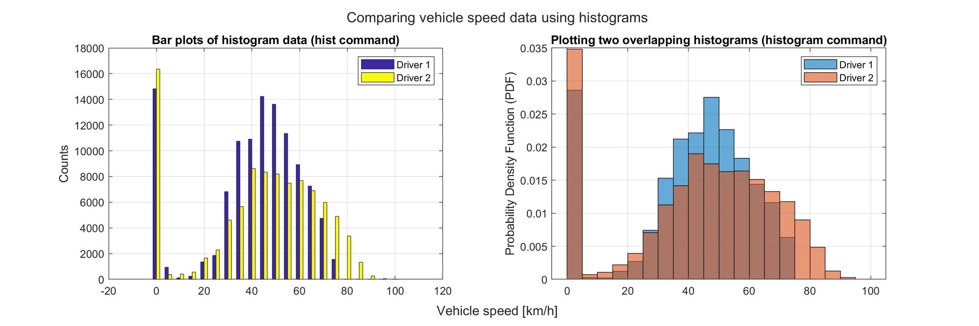
The histograms on the right side are normalized so that we can compare both files, even if the time of the second driver was shorter - which means that we have fewer data points. By dividing the counts of each bin by the size of the total sample, we actually get a representation of the discrete probability density function.

Analyzing the braking pressures

The histograms show that the second driver spent more time at speeds above 60 km/h than the first one. But both drivers were using exactly the same car. And the mean and median speed values are not that different between the two. So what could have changed? Perhaps it is also important to see how they were using the brakes.

%% Create histograms of the braking pressures
% This considers only the use of mechanical brakes.
% The electric car can also use the electric motors for regenerative braking. 
% This is enabled through a small portion of the brake pedal travel.
% These two particular datalogs do not contain information about that, so we will
% focus on the mechanical (hydraulic) brakes.

t1.BrakeFront(t1.BrakeFront <=0) = 0; %filter negative pressure values
t2.BrakeFront(t2.BrakeFront <=0) = 0; %filter negative pressure values
%%
figure;
hold on
histogram(t2.BrakeFront, 'Normalization', 'cdf')
histogram(t1.BrakeFront, 'Normalization', 'cdf')
set(gca,'YScale','log')
ylabel('cumcount (log scale)')
xlabel('Pressure [bar]' )
title('Brakes pressure in the front circuit ')
legend( 'Driver 2', 'Driver 1')
grid on

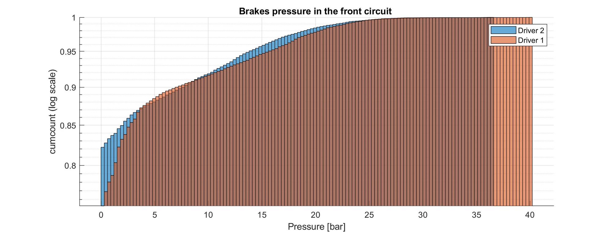
The bars on the left side represent the low-pressure values, which are the most common values present during driving. This makes sense since one doesn’t drive with the brakes pressed, especially during a race.

However, we can see that the number of times that the brakes were completely disengaged was lower for driver 1. This could mean that the first driver actually had the brakes slightly pressed constantly, perhaps without noticing. Driver 1 also pushed the brakes to higher pressures (up to 40 bar, which probably was the full-scale reading of the pressure sensor).

Let’s see also at what speeds the drivers were braking.

Finding the vehicle speeds at the start of the braking maneuvers

To do this, we need to identify the speeds at the start of the braking maneuvers. I defined a small pressure value to use as a threshold for identifying when the brakes are pressed. This is a bit of an iterative process - you don’t get it right the first time and need to adjust the value until the results make sense.

Let's use again the power of indexing, I don't want to wait forever with a for loop. We just need to determine in which rows there was a change in pressure that we could recognize as a pedal press. We also need to consider only the cases in which the vehicle was actually moving. So we have three conditions:

1. Low pressure on instant t
2. High pressure (greater than a threshold) on instant t+1
3. Vehicle speed greater than a minimum value at instant t+1

I indexed the tables using these three conditions and used parentheses to make them more readable (they are not really needed for the code to work). The trick is to impose the second and third conditions (t+1) by indexing the table from the second row. This creates the shift in time values that we would normally obtain using a loop with an increasing counter:

%% Find the index of the start of braking

%Define a pressure threshold value to consider as start of braking
p_start = 2; % bar

% Create indices for the start of the braking maneuvers
id_start1 = (t1.BrakeFront <= p_start) & ([t1.BrakeFront(2:end);0] > p_start) & ([t1.Veh_Spd(2:end); 0] >= 15);
id_start2 = (t2.BrakeFront <= p_start) & ([t2.BrakeFront(2:end);0] > p_start) & ([t2.Veh_Spd(2:end); 0] >= 15);

%% Verify that the identified points make sense
figure
plot(t1.Time_s, t1.BrakeFront, 'b', 'LineWidth', 1,'DisplayName', 'Pressure')
hold on
x = [t1.Time_s(id_start1), t1.Time_s(id_start1)];

% Show a black vertical line at the start of each braking maneuver
line(x, ylim, 'Color', 'k', 'LineWidth', .5, 'HandleVisibility', 'off'); 
yline(p_start, 'DisplayName', 'Brake start threshold' ,'LineWidth', 2) 
ylabel('Pressure [bar]' )
yyaxis right

plot(t1.Time_s, t1.Veh_Spd, 'r', 'LineWidth', 1, 'DisplayName', 'Vehicle Spd')
set(gca, 'Ycolor', 'r')
ylabel('Vehicle speed [km/h]')
xlabel('Time [s]' ), xlim([750, 800])
legend, grid on

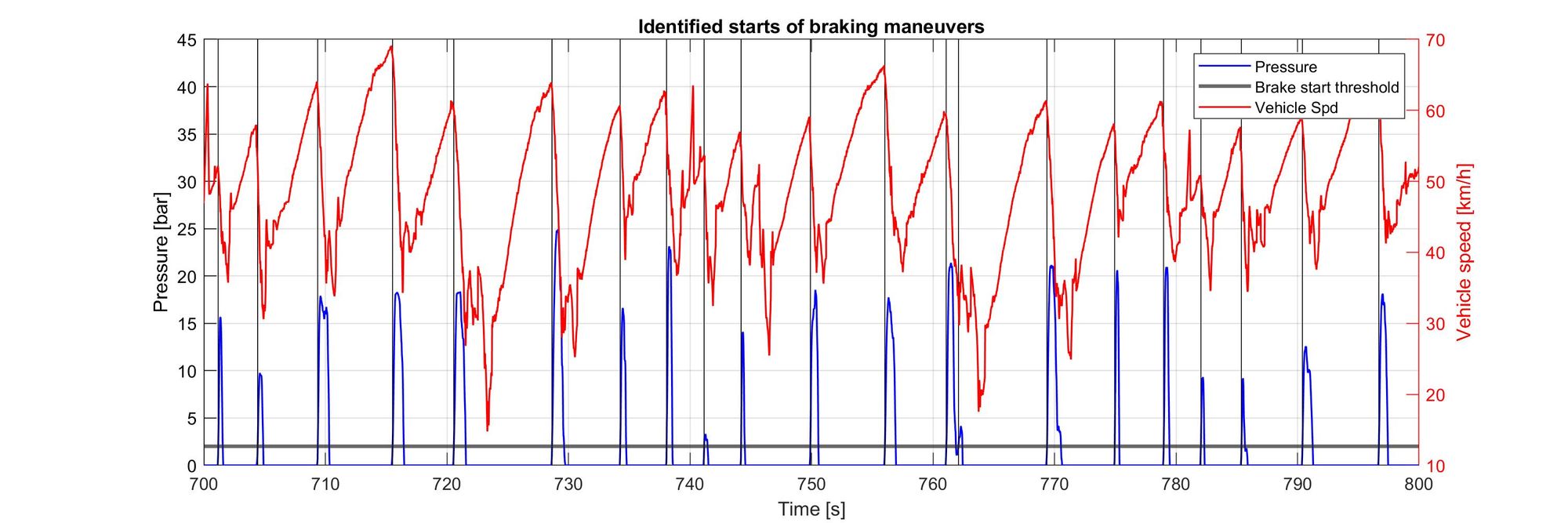
Great! we have identified the starts of braking maneuvers. Now let’s look at the speeds at which the drivers started braking. We just have to create histograms of the vehicle speeds using the indices we just found:

%% Create histograms and plot them
                                                
histograms = figure('Name', ['Histograms comparison'], 'Position', [10 10 900 600]);
title('MATLAB figure')
xlabel('Vehicle speed [km/h]')
binEdges = 10:5:100;

histogram(t1.Veh_Spd(id_start1), binEdges, 'Normalization' , 'probability')
hold on
histogram(t2.Veh_Spd(id_start2), binEdges, 'Normalization' , 'probability')
legend('Driver 1', 'Driver 2')
ylabel('Probability')
xlabel('Vehicle speed at the start of braking [km/h]')
grid on

Looking at the histograms, we can see that the first driver initiated more braking maneuvers between 60 and 70 km/h, but he also initiated more braking maneuvers at lower speeds - below 55 km/h. The second driver was braking at higher speeds.

Conclusion

This was a simple toy example of how to use MATLAB to do some tasks with real-world data. Besides plotting time series plots to visualize the two datasets, we used histograms to get valuable insights.

Sometimes we can be too concerned with the time-based evolution of the data we are looking at, and we miss details about their distribution or the trends and correlations between different variables.

Seeing how histograms can be easily used to get insights without actually needing to look at the times series can sometimes open a new perspective when looking at data recorded from physical things (cars, machines, sensors, etc).

Hopefully, this example was useful or interesting for you if you are just getting started doing similar things. I would be glad if it was in any way :)

In the next entry, I will repeat the analysis (at least the main part) using Python instead of MATLAB. Stay tuned!