Moving average filters: the good and the bad

Moving averages are easy to implement, they seem easy to use (just adjust the window size until you get good-looking, smooth lines), and they are available as easy-to-find functions in most data analysis tools.

Yet, they are not exactly the best choice for all situations.

As with any digital filter, using the wrong filter parameters can lead you to remove information you will actually need, or maybe not remove anything at all. You’d be surprised, but these two extreme cases do happen in real life.

Here, I'm going to share some notes about the moving mean or moving average filter.

Moving Average filter properties

💡 It’s a convolution of the input signal with a rectangular pulse having an area of one.

🔎The noise is reduced by a factor equal to the square root of the number of samples in the moving window.

Pros:

• Easy to implement
• Great for signals encoded in the time domain
• Remove random noise
• Keep fast step response

Cons:

• Causal filter: introduces lag (inevitably)
• ⚠️ Terrible for filtering data in the frequency domain. It’s a Low-Pass filter with sub-optimal attenuation.

Example uses:

✅Filtering noise from slow-changing signals, like the temperature of some heavy machinery.

❌Processing data containing relevant frequency information (i.e. the accelerations of a car suspension, sound, etc.)

Here's how this kind of filter is implemented. I'm using MATLAB for demonstration purposes, but the concept is the same in any programming language. Just be aware that Matlab is one-indexed.

% Filter raw data using a moving average filter

% Implement the filter using custom code

k = 50;   % Window size in number of samples
          % The value to be used needs to be decided case-by-case

filt_data = zeros(length(signal),1); % Initialize array of filtered data

for i = k+1:n-k+1

    % Each point is the average of the neighboring k points
    %                   |<---------- mean --------->| 
    %...| i-k-2 | i-k-1 | i-k | ... | i | ... | i+k | i+k+1 | i+k+2 | ...
    
    filt_data(i) = mean(raw_data(i-k/2:i+k/2));

end

% If you implement your own function, you'll have to find a way to 
% deal with the start and end of the filtered data
% You can implement a shrinking window size, for example

% Using Matlab's function
filt_data_funct = movmean(raw_data, k);

The number of samples used for the window size determines the frequency response of the filter.

A larger value of N will produce a filter with a narrower passband in the frequency domain. In other words, it will let pass only the lowest frequencies, reducing the amplitude of higher frequencies. In the time domain, this looks like “smoother” data.

This is great if the underlying signal does not include any relevant frequency information. We will essentially filter out (part of) the measurement noise.

Here’s how we can calculate the frequency response of a moving average filter:

N = 20; % Window size (number of samples)
f = 0:0.001:0.5;

H1 = sin(pi*f*N)./(N*sin(pi*f));
H2 = sin(pi*f*N/2)./(N/2*sin(pi*f));
H3 = sin(pi*f*N/5)./(N/5*sin(pi*f));

This might be undesired if we wanted to analyze high-frequency content in the signal. In such case, we might want to use a high-pass or even a band-pass filter.

A practical example

Let’s suppose we want to measure some signal containing both low and high-frequency information.

For this example, I will create a signal combining sine waves with frequencies of 0.5 Hz and 100 Hz. This will be our “true” process data.

I will also add some random noise to simulate some noisy measurement data. This will be the data we would have to work with if we were collecting information about this system with some imperfect (real) sensors.

%% Define sampling time and time vector
ts = 0.001; % s, sampling time
time(:,1) = 0:ts:10;
n = length(time); % number of samples

% Make some noise
rng(42);
noise(:,1) = randn(n, 1);
amp = 2; % Noise amplitude

% Create "true" signal and raw data
f1 = 0.5;  % Hz
f2 = 100;    % Hz
signal = sin(2*pi*f1*time) + sin(2*pi*f2*time + .3);
raw_data = signal + amp*noise

Now I will apply a moving average filter to this signal, in an attempt to remove the noise. Let’s see if we can recover the original information by doing this.

I’ll use 10 and 50 samples for the window size, just to illustrate the difference.

At first sight, it seems that using a 50-sample window size did filter a good part of the noise.

If we increased the window size to a large number like 400 samples, we would get a much smoother sinusoid with a frequency of about 0.5 Hz.

However, when we zoom in and compare the results with the original signal, we can see that the high-frequency content is not well represented. The filter with a 10-sample window did not work very well either.

Ok, this is an exaggerated example. But I think it illustrates the idea.

If we did a quick frequency analysis, we could effectively see that the energy in the frequency of 100 Hz almost disappeared.

% Amplitude spectrum of original signal
amp_signal = fft(signal);
amp_signal = 2*abs(amp_signal)/n;

% Amplitude spectrum of raw data
amp_data = fft(raw_data);
amp_data = 2*abs(amp_data)/n;

% Amplitude spectrum of filtered data (k)
amp_filtd_1 = fft(filt_data_k);
amp_filtd_1 = 2*abs(amp_filtd_1)/n;

% Amplitude spectrum of filtered data (k/5)
amp_filtd_2 = fft(filt_data_k_5);
amp_filtd_2 = 2*abs(amp_filtd_2)/n;

% Vector of frequencies in Hz
nyquist_freq = 1/ts/2; % Nyquist sampling theorem
freq = linspace(0,nyquist_freq, floor(n/2)+1);

% nexttile
figure;

hold on
plot(freq, amp_signal(1:length(freq)),'r', DisplayName= 'signal')
plot(freq, amp_data(1:length(freq)), 'k', DisplayName= 'raw data')
plot(freq, amp_filtd_1(1:length(freq)), 'b', DisplayName= ['filtered data with ' num2str(k,2) ' samples window size'])
plot(freq, amp_filtd_2(1:length(freq)), 'g', DisplayName= ['filtered data with ' num2str(k/5,2) ' samples window size'])

grid minor
xlabel('Frequency [Hz]')
ylabel('Amplitude')
set(gca, 'YScale', 'log')
xlim([0 150])
legend('Location', 'south')

We can even see the attenuation effect shown in the previous figure when we looked at the filter's response.

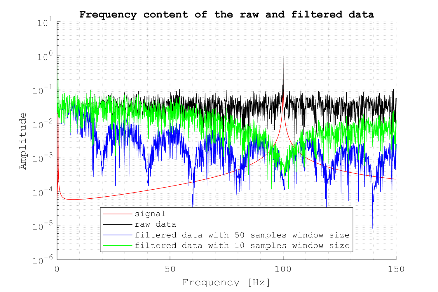
So in this case, using a moving average filter would be OK if we only care about the low-frequency content. With a large window size, the sine wave would look great.

But in real life signals don't always represent smooth processes. Even if a process is slow most of the time, using a very large window to smooth out a signal is not a good idea. This is because the larger the window you use,  the greater the delay introduced in the filter: it uses more previous samples to compute the next value.

If for any reason the input changes quickly (an "event" happens), it will take you some time to see that reflected in your filtered signal. This can be bad for control strategies, for example.

Conclusion

I just shared a refresher on the properties of a moving average as a digital filter. It was a good exercise for me, and I hope you have a clearer idea about what this filter can and cannot do. Hopefully, we'll be more conscious of this the next time we decide to smooth out some measurement data.

In my case, I ask myself: could there be some higher frequency information I’d be cropping out if I apply a moving average filter? For signals representing slow-varying processes, this is not an issue, but in other cases, you might need to consider it.

References

The Scientist and Engineer's Guide to Digital Signal ProcessingSignal processing problems, solved in MATLAB and in Python