Leveraging data aggregations in Python: using Pandas groupby method for data analysis

SQL and spreadsheet thinking to level up your Pandas game

When analyzing data as a beginner in Python programming, I would often write for loops or complicated functions to achieve things I could do faster using Pandas’ groupby method, especially when computing data aggregations.

The problem was I didn’t fully understand how it worked and how powerful it was.

But working with spreadsheets and SQL helped me get a better grasp of what it does. Yes, I learned from Excel tips and the kind of things I thought I wanted to move away from.

So here I’m going to share how I understood better what Pandas’s groupby method does, and how we can benefit from it, using a few examples.

What are data aggregations?

Aggregations are computations we use to obtain information about a potentially large amount of data points.

Think about it like a summary.

When we use methods like max(), min(), sum(), mean() and median(), they return a single number that provides usefull information about a whole column or row. Those are some of the basic data aggregation methods.

They are easy to understand because we think about them like we were taught in school: “to compute the mean, take the sum of all the elements divided by how many elements you have”.

Pandas dataframes are, essentially, tables. So many of the methods they provide for data aggregation are very similar to Excel and SQL.

In particular, groupby reminds of Excel’s pivot tables and SQL’s own GROUP BY clause.

Split, apply, and combine

This is the mantra I tell myself whenever I’m struggling to understand how a groupby operation works. Essentially, we can see the output of a groupby as the result of three simpler operations that are done sequentially.

These are illustrated in the figure below.

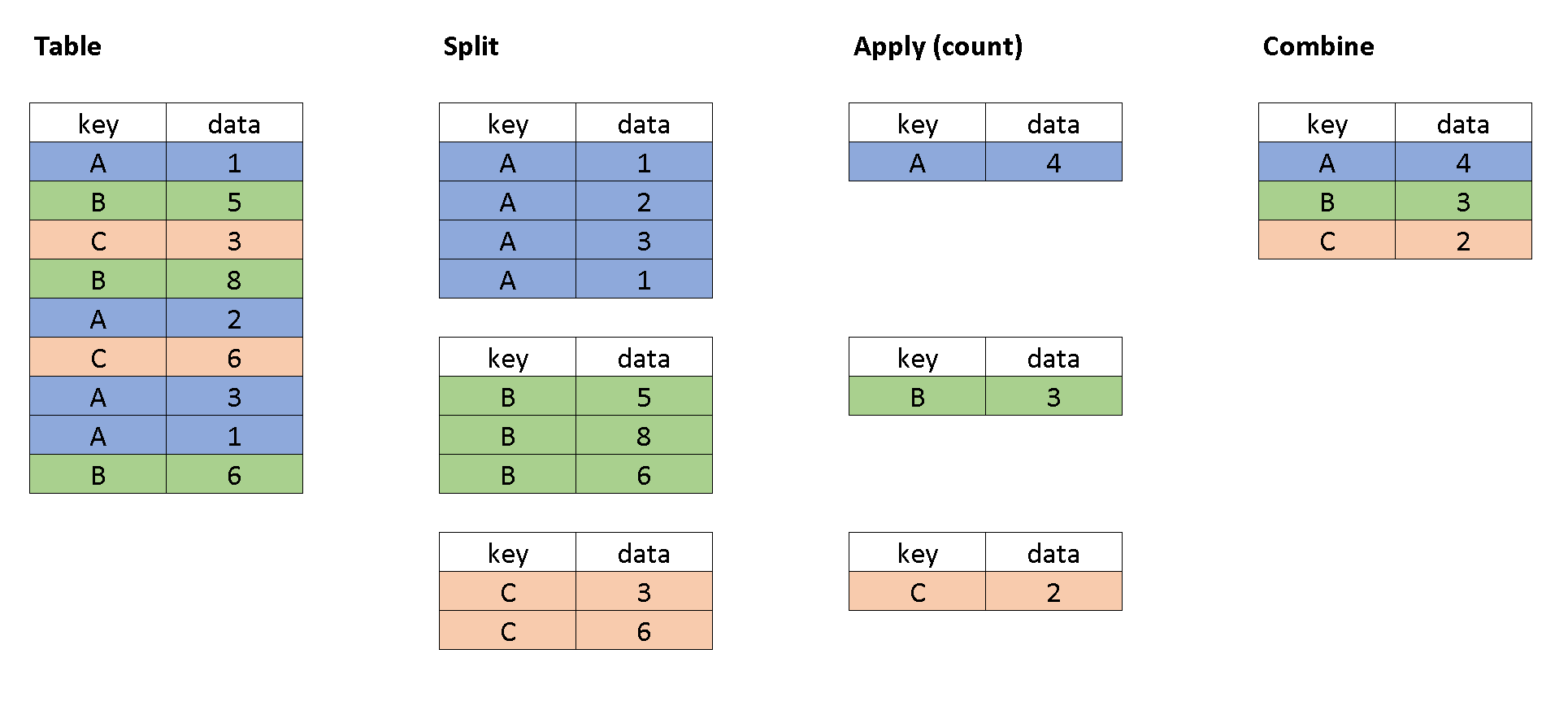
First, we split the data into parts according to the keys we pass as an argument to the groupby method.

Next, we apply the desired aggregation to each one of the parts, separately. For instance, we count them, or take the mean value of them, or any other computation we want.

Finally, we combine the results in a new, aggregated table which shows the computation result for each sub-group.

It becomes easier to understand when you think of the operation as a sequence of steps. At least it did for me.

Why aggregations are powerful when analyzing data?

To illustrate how powerful this is, let's start with an example data frame.

Let’s say we are analyzing data for some business and we have a dataset about customer transactions. We can create a synthetic dataset just for testing:

import pandas as pd
import numpy as np
import time

# Generate a large synthetic dataset with 10k rows
num_rows = 10000
data = {'CustomerID': np.random.randint(1, num_rows/4 + 1, num_rows),
        'TransactionID': np.arange(num_rows),
        'Revenue': np.random.rand(num_rows) * 100}

transactions = pd.DataFrame(data)
transactions.head()

Out[1]: 
				   CustomerID  TransactionID    Revenue
				0          55              0  31.403065
				1         198              1  59.796718
				2        2431              2  22.002152
				3         960              3   3.743878
				4         120              4  40.094364

Now, imagine we want to know the total revenue for each customer. We could get the results by using a for loop:

def extract_with_for_loop(df):

    revenue_by_ID = pd.DataFrame(
                          columns=['CustomerID', 
                          'TotalRevenue'])

	for customer in df.CustomerID.unique():
		transactions = df[df.CustomerID == customer]
		revenue_by_ID = revenue_by_ID.append(
                              {'CustomerID' :customer, 
							  'TotalRevenue' : transactions.Revenue.sum()}, 
							   ignore_index = True)
                               
	revenue_by_ID = revenue_by_ID.sort_values('CustomerID')
				
	return revenue_by_ID


start_time = time.time()
rint(extract_with_for_loop(transactions).head())
end_time = time.time()
print('Time taken using for loop:', end_time - start_time, 'seconds')


Out[2]:    CustomerID  TotalRevenue
				0         1.0    197.259255
				1         2.0    179.829982
				2         3.0    152.390251
				3         4.0    313.157241
				4         5.0    109.242505
				Time taken using for loop: 9.578813314437866 seconds

But what if I told you we can use indexing to do exactly that with a single line of code, and much faster?

# Define another function to extract the same data, this time using groupby
def extract_with_groupby(df):
    revenue_by_ID = df.groupby('CustomerID')['Revenue'].sum().reset_index(name='TotalRevenue')
    return revenue_by_ID

# Test the time when using groupby
start_time = time.time()
print(extract_with_groupby(transactions).head())
end_time = time.time()
print('Time taken using groupby:', end_time - start_time, 'seconds')


Out[3]:    CustomerID  TotalRevenue
				0           1    197.259255
				1           2    179.829982
				2           3    152.390251
				3           4    313.157241
				4           5    109.242505
				Time taken using groupby: 0.01568460464477539 seconds

That is awesome! less typing, and we obtained the same results in a fraction of time.

But why would I want to mess with conditions and indexing if I can just wait a few seconds more?

Well, I’m glad you ask…

What happens when you have more data?

The problem with using for loops to do this kind of data extraction is that your code will need to go through each row and apply the conditional statement individually.

This means that execution time will grow as the size of your dataset grows.

Let’s measure that.

Now, I’m going to do something contradictory. I will prove how slow for loops can be, by using a for loop!

I'll create 10 dataframes with increasing sizes, and use timeit to measure the execution time of the two functions I showed above when running them 5 times for each dataframe size.

# Test the performance of the two methods for varying DataFrame sizes
import matplotlib.pyplot as plt
import timeit



df_sizes = np.linspace(100, 10000, num=10, dtype=int)
indexing_times = []
for_loop_times = []

for size in df_sizes:
    # Create example dataframes with varying sizes for each iteration
    data = {'CustomerID': np.random.randint(1, size/4 + 1, size),
            'TransactionID': np.arange(size),
            'Revenue': np.random.rand(size) * 100}

    df = pd.DataFrame(data)
    
    indexing_time = timeit.timeit('extract_with_groupby(df)',
                                  setup='from __main__ import extract_with_groupby, df',
                                  number=5)
    indexing_times.append(indexing_time)
    
    for_loop_time = timeit.timeit('extract_with_for_loop(df)',
                                  setup='from __main__ import extract_with_for_loop, df',
                                  number=5)
    for_loop_times.append(for_loop_time)

# Plot the results
fig = plt.figure(figsize= (8,6), dpi = 72)
ax = fig.add_subplot(1,1,1)
ax.plot(df_sizes, indexing_times, label='Indexing')
ax.plot(df_sizes, for_loop_times, label='For Loop')
ax.set_xlabel('DataFrame Size')
ax.set_ylabel('Execution Time (Seconds)')
ax.set_title('Execution Time Comparison for DataFrame Extraction')
ax.legend(frameon = False)
plt.tight_layout()
fig.show()
fig.savefig('comparison.png', dpi = 300)
print('Created figure')

As you can see, the for loop version of this code is much slower than the indexing version, especially for large data sets.

This is because the for loop requires iterating over every row in the data frame and performing the calculation for each customer individually, whereas indexing allows us to select and manipulate large groups of data at once, making it much faster and more efficient.

Conclusion

Aggregations are the bread and butter of many Data Analysis workflows, and they become more important as the amount of data we handle grows.

Sadly, though, as a Mechanical Engineer coming from Matlab, it took me time to realize this.

Working with tables and aggregations seemed more suitable for people analyzing different kinds of data, like in finance, marketing, sales or insurance companies.

Certainly not data coming from physical systems (which is the only thing I used to work with).

But I was wrong. If you are interested, I’ve written before about how I leveraged it in my job when analyzing data from a test bench.

I hope this short post helped you get a better understanding of Pandas groupby method, and how you can use it to avoid time-consuming tasks and improve the efficiency of your data analysis.

Have a good one!

Check out my other posts for more insights about using and learning Python for tasks you’d usually do with Matlab, or just general tips about Data Analytics and programming.

Consider subscribing (it's free! and I hate spam) to receive new posts about these topics.