DL Notes: Gradient descent
I describe the algorithm of gradient descent, which is used to adjust the weights of an ANN. A summary of information from different sources that I used when studying this topic.

How Neural Networks "Learn"
Artificial Neural Networks (ANNs) are universal function approximators. They can approximate any complex function if provided with enough data, have a proper architecture, and are trained for enough time.
But what does “training” a network even mean?
In a previous post about the feedforward process, I mentioned that training a network means adjusting the value of its weights, to obtain a better fit of the function we are trying to approximate.
In this post, I’m going to describe the algorithm of gradient descent, which is used to adjust the weights of an ANN.
Let’s start with the basic concepts.
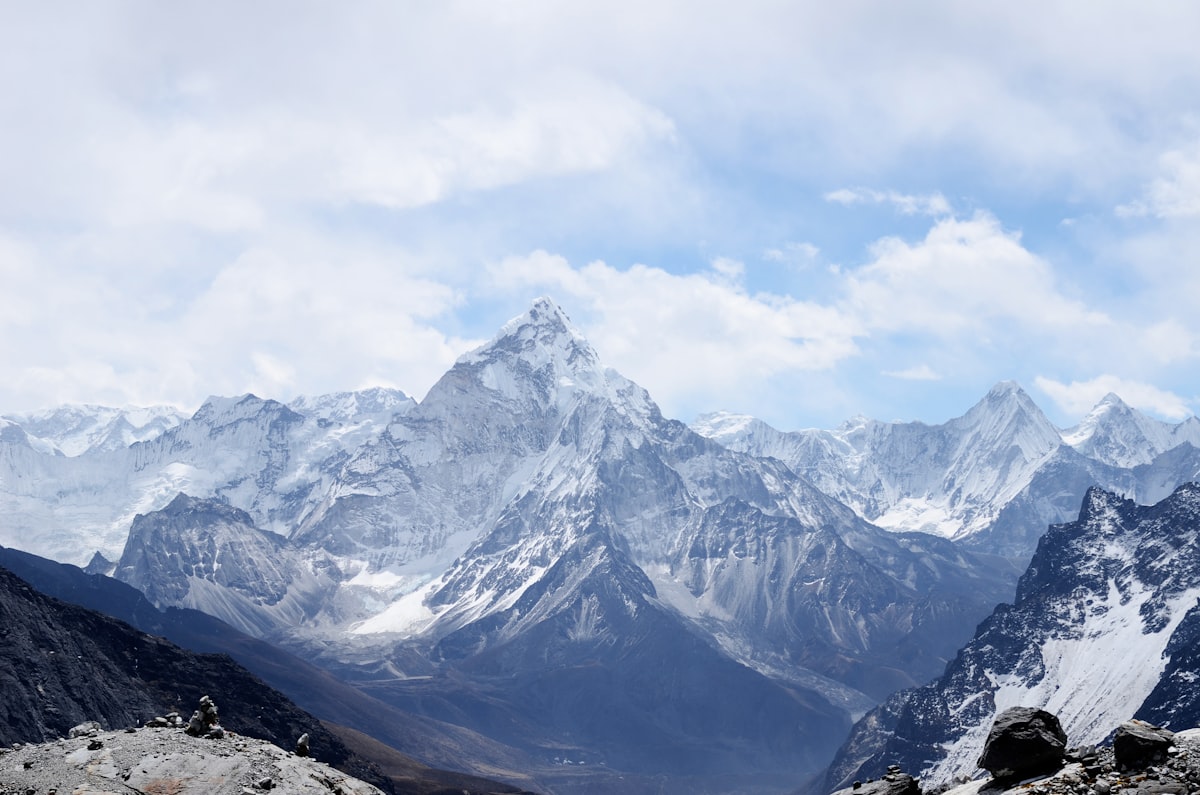
Descending from a mountain
Imagine we are at the top of a mountain and need to get to the lowest point of a valley next to it.
We don’t have a map, it is foggy and getting dark, we lost the routes and need to get to the bottom quickly. Not a nice scenario, but it shows the “boundaries” of the problem.
For our safety, let’s suppose there are no steep ridges in the mountain, so it is similar to a differentiable function.
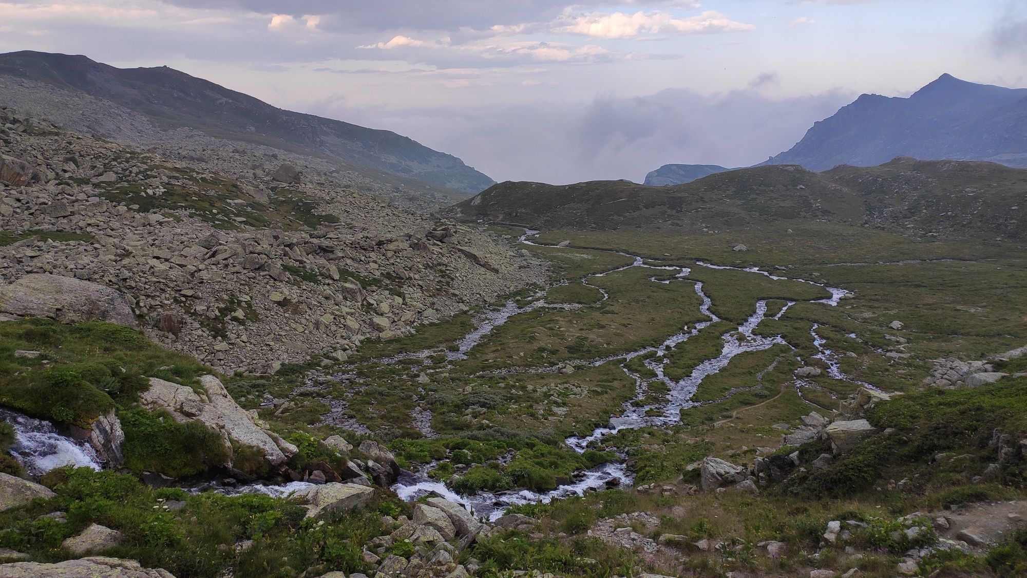
When it gets dark, we can’t see in which direction we are moving. The only way we can descend is by taking small steps, and checking whether we are at a lower height or not.
If we notice we moved up, we go in the opposite direction. If we moved down, we continue that way. We repeat the process until, eventually, we’ll reach the bottom.
As you can see, this is not necessarily the best approach. We might end up in a small valley, not at the bottom of the mountain, or we could spend a huge amount of time on a plateau.
This illustrates the basic working principle of gradient descent and also its main challenges. We’ll come back to this example, but let’s see a more formal explanation first.
What is a gradient?
A gradient is a representation of the rate of change of a function. It indicates the direction of the greatest increase or decrease. Intuitively, that means the gradient is zero at a local maximum or a local minimum.
For a function that depends on several variables (or coordinate axes), the gradient is a vector whose components are the partial derivatives of the function, evaluated at a given point. This is denoted with the symbol ∇ (nabla) which represents the vector differential operator.
Let’s see this in math notation. Suppose we have an n-dimensional function f:
$$ f(x_1, x_2, ... ,x_n) \ \ \ \ \ \ f:\R^n \rightarrow \R $$
The gradient of this function at point p (which is determined by n coordinates), is given by:
$$ \nabla f (p) = \left[\frac{\partial f}{\partial x_1} , \frac{\partial f}{\partial x_2} , ..., \frac{\partial f}{\partial x_n} \right]^T \ \ \ \ \ \ \nabla f:\R^n \rightarrow \R^n $$
Coming back to the example of the mountain, there are areas of the mountain where the terrain is steep, like the mountain slopes, and other zones where the terrain is almost flat, like a valley or a plateau. Valleys and plateaus represent local minima, which are usually critical points.
The gradient descent method
For many optimization problems, we aim to minimize a loss function to achieve the most accurate result.
$$ \theta^* = arg\ min_\theta J(\theta) $$
In Deep Learning and ANNs, the loss functions we use are differentiable: they have no discontinuities, being smooth across their whole domain.
This allows us to use the derivative of the loss function with respect to the independent variables as an indication of whether we are moving towards a solution (a global minimum).
How large are the steps we take in proportion to the derivative? this is determined by a step size parameter, \(\eta\) (we can call it learning rate when we are talking about Deep Learning). It will multiply the gradient, scaling it to determine the step size.
This way, steeper gradients will produce larger steps. As we approach a local minimum, the slope (gradient) will tend to zero.
Let’s look at the following figure, for example, to illustrate how this works when optimizing a 1D function:
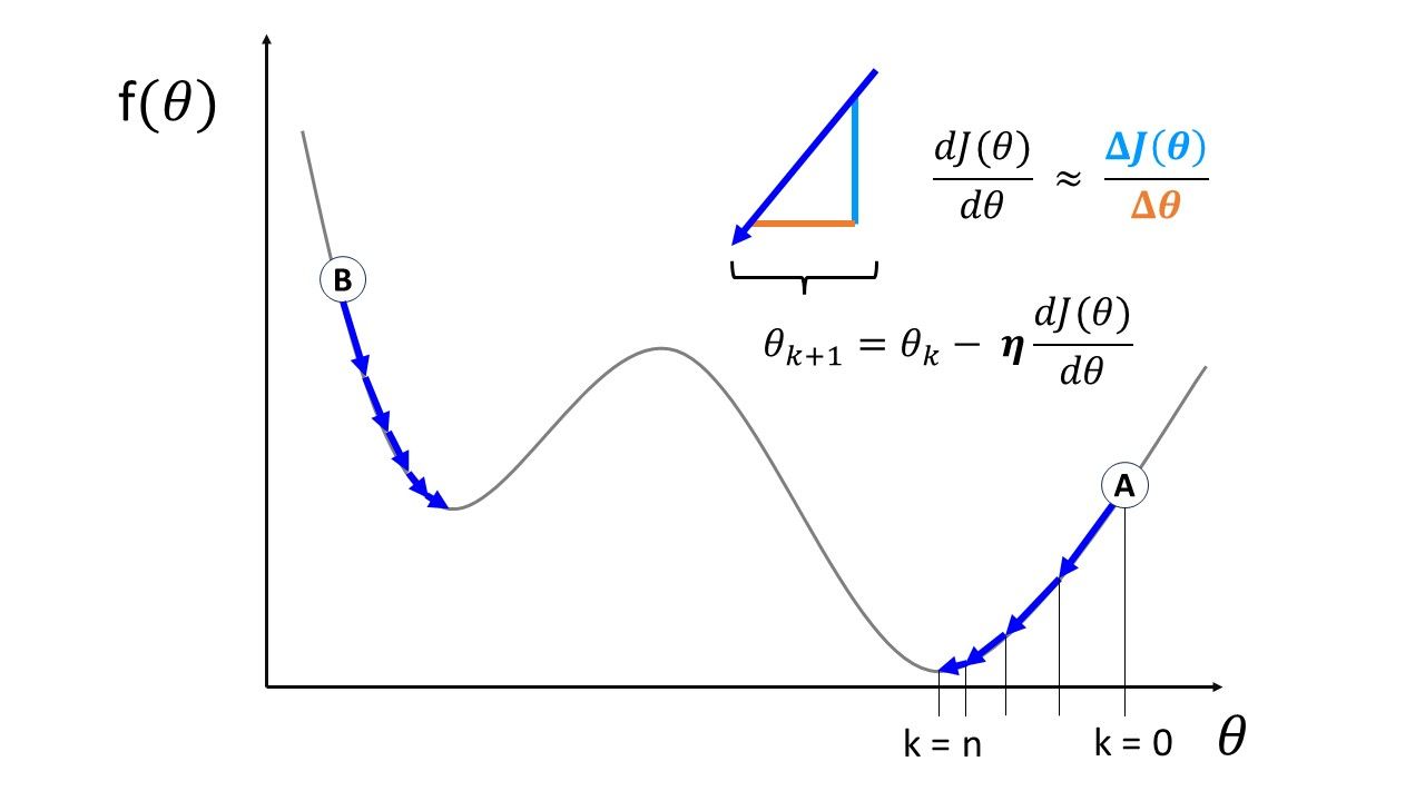
As you can see, we initialize our “search” for the minima at an arbitrary point (I’ve depicted two examples, A and B). We gradually take steps toward the closest minima, making changes in \(\theta \) in proportion to the slope.
The illustration represents what the following algorithm does (pseudo-code) [1]:
θ(0) = θ_init       # Initialization of optimization variable
η = 0.02            # Arbitrary step-size parameter
Є = 0.01            # Optimization accuracy
k = 0               # Iteration counter

while |f(θ(k+1) - f(θ(k))| > Є:
	θ(k+1) = θ(k) - η ∇f(θ(k))
	k = k + 1
The loss function here is like our example of the mountain when it’s dark and we don’t have a map: we don’t know what it looks like. We want to know the value of \( \theta \) for which \( J \) is minimized, but the optimization algorithm doesn’t know what the value of \( J \) would be for all possible inputs \( \theta \) .
This is why we initialize our optimization algorithm with any arbitrary value of \(\theta \). For instance, points A and B in the figure represent two different initialization values.
Potential problems with Gradient Descent
The gradient descent algorithm is effective because it can help us obtain an approximate solution for any convex function.
If the function we are trying to optimize is convex, for any value of \( \epsilon\) there is some step size \( \eta \) such that gradient descent will converge to \(\theta ^*\) within \( \epsilon\) of the true optimal \( \theta \) . [1]
However, as you might have guessed, this is not perfect. The algorithm might converge, but that doesn’t guarantee that we’ll find a global minimum.
The main challenges of gradient descent are the following:
Arbitrary initialization has an impact on the results
Using different initialization values, we could encounter local minima instead of global minima.
For example, starting at point B instead of point A in the previous figure above.
Or, a less evident case, converging to a plateau (vanishing gradient problem) as shown by the blue line in the figure below.
Selecting the appropriate step size requires a trade-off between convergence speed and stability
There’s an interaction between the step size or learning rate, and the number of epochs we should use to achieve accurate results.
Take for example the results of a parametric experiment, shown below. The images are from the online course A Deep Understanding of Deep Learning, by Mike X Cohen, which I highly recommend to anyone interested in Deep Learning and using PyTorch, following a scientific approach.
In this case, Mike showed how to test the results for a gradient descent optimization when changing the learning rate and the number of training epochs independently (one parameter over time, for a grid of different values). We can see how both parameters affect the results for this particular case.
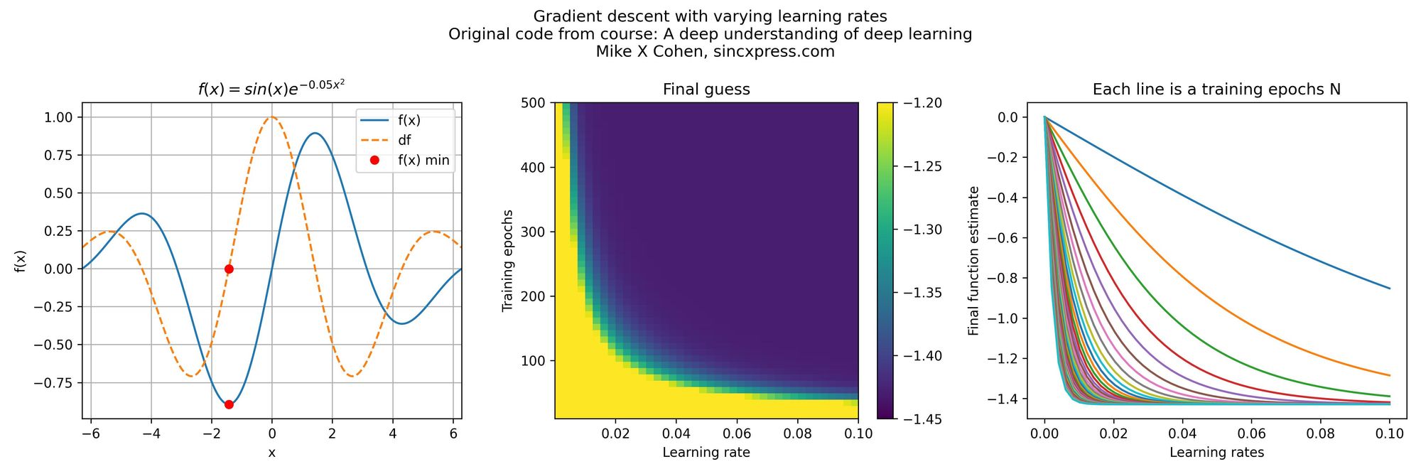
The true global minimum of the function is around -1.4. You can see that for smaller learning rates, it takes a larger number of training epochs to converge to that result. So it would seem like just using a larger learning rate can help us reduce the computational time.
But in practice, this isn’t a simple matter of convergence speed.
Large step sizes can lead to very slow convergence, prevent the algorithm from converging at all (oscillating around the minima forever), or provoke a divergent behavior.
The next figure shows how different learning rates affect the results of the optimization, even if we initialize the algorithm in the same location \(x = 2\).
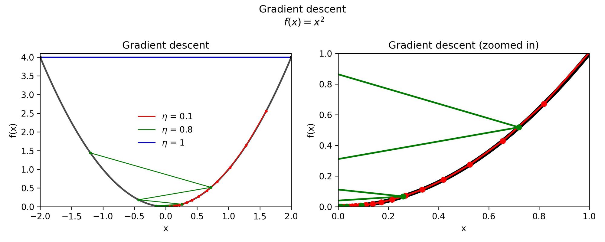
Here, it is evident that having large step sizes improves the convergence speed but only up to a certain point.
Increasing the learning rate by an order of magnitude caused the algorithm to get stuck. The results for \(\eta = 1\) oscillate between \(x =2\) and \(x = -2\), and this is shown only by the blue horizontal line in the left figure.
In some cases, a large step size might actually “shoot” the results to infinity, causing a numerical overflow of our program.
On the other hand, too small step sizes can create a very slow convergence or no convergence at all.
Gradient descent for training a Neural Network
In the context of Deep Learning, the function we are trying to optimize is our loss function \(J\). We define our training losses as the average of the losses for all our training dataset:
$$ TrainLoss(\bold w) = \frac{1}{Dtrain} \sum_{(x,y) \ \in \ Dtrain} J(x,y,\bold w) $$
Where Dtrain is the number of samples in our training dataset.
Thus, we can implement gradient descent based on the following algorithm, in which we compute the gradient of the training losses with respect to the weights for a certain number of epochs to perform an update of the model weights [2]
w = [0, ... ,0]    # Initialize the weights
for k = 1,..., n_iters:          # Repeat for n iterations
  grad = ∇w TrainLoss(w)         # Gradient of the Training losses

  w[k] <-- w[k-1] - η * grad     # Update the model weights
Since we are computing an average of the gradient of the loss function, we have a better estimate of it. For this reason, the weights update is more likely to be in the direction that improves the model performance.
The problem with this implementation of gradient descent is its low speed.
For a toy example with a few points and a simple function it might work well, but imagine we are developing an ANN and we have a million data points to train it.
To train the ANN with this algorithm, we would need to compute the outputs of the model for each sample of the training data and then average their losses as a large batch. Just to do one update of the weights. Then repeat it, over and over again, until we reach convergence.
This is called Batch Gradient Descent. It makes one (accurate) weight update per iteration, but each iteration can take a long time because we are repeating the model computation n times.
To overcome this problem, we could use the so-called Stochastic Gradient Descent algorithm.
Stochastic Gradient Descent
To overcome the slow convergence problem of Batch Gradient Descent, we can perform an update of the model weights based on each sample of the training set. The advantage is that we don’t need to wait until we have looped through the whole set to perform just one update of the weights.
We can do this by using the Loss function for each individual sample, instead of the whole training losses.
This is what the Stochastic Gradient Descent Algorithm (SGD) looks like
w = [0, ... ,0]                          # Initialize the weights
for k = 1,..., n_epoch:
    for (x, y) ∈ Dtrain:                 # For each sample
        grad = ∇w J(x,y,w)
        w[k] <--  w[k-1] - η(k) * grad   # Update the model weights
Notice that the step size is a function of the training iterations. That’s because, for the algorithm to converge, η must decrease as the number of iterations progresses.
In the lecture notes of MIT 6.036 [1], the following theorem is mentioned:
Theorem 4.1. If J is convex, and η(t) is a sequence satisfying
$$ \sum_{t=1}^{\infty}\eta(t) = \infty \ \ and \ \ \sum_{t=1}^{\infty}\eta^2(t) < \infty $$
then SGD converges with probability one to the optimal \(\theta\).
People take different approaches to reduce the value of η as the training progresses, and this is often called “Annealing”:
- Changing the learning rate in proportion to the training epoch (for instance, η(t) = 1/t) , or setting it to a smaller value once a certain learning epoch has been reached. This method offers good results but is unrelated to the model performance. This is called “learning rate decay”, and is the industry standard to handle this problem.
- Multiplying the learning rate by the gradient of the loss function: This method is good because it’s adaptive to the problem, but requires careful scaling. This is incorporated into RMSprop and Adam variations of gradient descent.
- Multiplying the learning rate by the losses: The advantage is that this is also adaptive to the problem, but requires scaling too.
SGD may perform well after visiting only some of the data. This behavior can be useful for relatively large data sets, because we may reduce the amount of memory needed, and the total runtime compared to the “vanilla” implementation of gradient descent.
The Batch implementation is slower because it needs to run through all samples to perform a single update of the weights.
SGD performs an update at every sample, but the quality of the updates is lower. We may have noisy data or a really complex function we are trying to fit with our ANN.
Using a batch of size Dtrain is slow, but accurate, and using a batch of size 1 is fast, but less accurate.
There is a term in between, and it’s called “mini-batch” gradient descent.
Mini-Batch Gradient Descent
If we split our data into smaller batches of equal size, we could do what Batch gradient descent does, but for each of those mini-batches.
Let’s say we divide the data into 100 smaller parts.
We go through our data in 100 steps. On each step, we look at the Training Losses just for the data contained in the current mini-batch and improve our model parameters. We repeat this until we have looked at all samples, and start the cycle again.
Each cycle is known as an epoch. I have used the term more loosely before just to refer to the number of iterations during optimization, but the normal definition refers to each cycle through the training dataset. For Batch gradient descent, an iteration is an epoch.
When we set how many epochs we want to use for training an ANN, we are defining how many passes through the training dataset we will make.
The advantage of using mini-batches is that we update our model parameters on each mini-batch, rather than after we have looked at the whole data set.
For Batch gradient descent, the batch size is the total number of samples in the training dataset. For mini-batch gradient descent, the mini-batches are usually powers of two: 32 samples, 64, 128, 256, and so on.
SGD would be an extreme case when the mini-batch size is reduced to a single example in the raining dataset.
The disadvantage of using a mini-batch gradient in our optimization process is that we incorporate a level of variability - although less severe than with SDG. It is not guaranteed that every step will move us closer to the ideal parameter values, but the general direction is still towards the minimum.
This method is one of the industry standards because by finding the optimal batch size, we can choose a compromise between speed and accuracy when dealing with very large datasets.
Thank you for reading! I hope this article was interesting and helped you clear some concepts. I’m also sharing the sources I used when writing this, in case you are interested in going through deeper and more formal material.
In a future post, I’ll write about more advanced methods of gradient descent (the ones people use in real applications) and how we actually update the model weights during training, using backpropagation, as gradient descent is only one part of the full story.
References
[1] MIT Open Learning Library: 6.036 Introduction to Machine Learning. Chapter 6: Gradient Descent
[3] Online course A Deep Understanding of Deep Learning, by Mike X Cohen (sincxpress.com)
[4] Standford Online: CS231 Convolutional Neural Networks for Visual Recognition