DL Notes: Advanced Gradient Descent
I researched the main optimization algorithms used for training artificial neural networks, implemented them from scratch in Python and compared them using animated visualizations.


In my previous article about gradient descent, I explained the basic concepts behind it and summarized the main challenges of this kind of optimization.
However, I only covered Stochastic Gradient Descent (SGD) and the "batch" and "mini-batch" implementation of gradient descent.
Other algorithms offer advantages in terms of convergence speed, robustness to “landscape” features (the vanishing gradient problem), and less dependence on the choice of learning rate to achieve good performance.
So today I’ll write about more advanced optimization algorithms, implementing them from scratch in Python and comparing them through animated visualizations.
I’ve also listed the resources I used for learning about these algorithms. They are great for diving deeper into formal concepts.
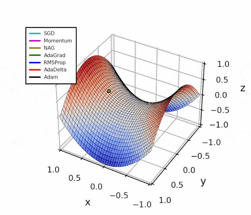
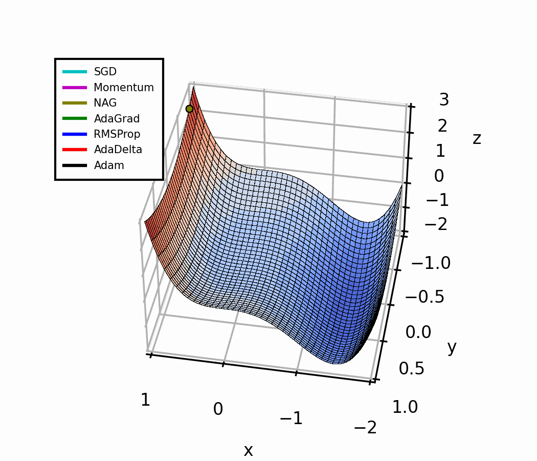
Comparing the algorithms using a simple objective function
Throughout this post, I’ll show how I implemented the different algorithms in Python.
I’ve created a Jupyter Notebook that you can access on GitHub or directly on Google Colab to see all the code used to create the figures shown here.
![]()
To generate the animations, I used the approach shown in my previous post about creating an animated gradient descent figure in Python.
The function definitions assume that the following code has been already included, as they use numpy classes and methods and call both the function f and its gradient, grad_f.
import numpy as np

# Create a function to compute the surface
def f(theta):
  x = theta[0]
  y = theta[1]
  return x**2 - y**2

# Define a function to compute the gradient
def grad_f(theta):
    returnValue = np.array([0.,0.])
    x = theta[0]
    y = theta[1]
    returnValue[0] += 2*x
    returnValue[1] += - 2*y
    return returnValue
Momentum

We could compare the optimization algorithm with a ball rolling downhill.
If the “ball” had momentum like it has in real life, it would be less likely to remain stuck in a local minimum after accelerating down the hill at full speed.
That’s what people realized when dealing with the problem of gradient descent getting stuck in local minima.
From high school physics, we know that translational momentum is defined by the product of the mass of an object and its velocity:
$$ \vec p = m \vec v $$
We also know that the gravitational potential energy of an object of mass $m$ is proportional to the height $h$ at which it is placed:
$$ U = mgh $$
Moreover, there is a direct relationship between the potential energy of an object and the force exerted on it
$$ \vec F = - \nabla U $$
The relationship between \(\bold p\) and \(U\) can be derived from Newton’s second law of motion:
The change of motion of an object is proportional to the force impressed; and is made in the direction of the straight line in which the force is impressed.
$$ \vec{F} = \frac{d\vec{p}}{dt} = m \frac {d \vec v}{dt} $$
How to add momentum?
When we initialize the optimization algorithm, we place the “ball” at a height \(h\), giving it potential energy \(U\).
The force exerted on the ball is proportional to the gradient of such potential energy. Like the gradient of the function we are optimizing (the surface over which we are moving).
The way momentum works for the optimization is by using the gradient to change the “velocity” of the particle, which in turn changes its position.
$$ \begin{align*} v_{t+1} &= \red{\mu v_t} - \eta \blue{\nabla f(\theta_{t}) }\\ \theta_{t+1} &= \theta_{t} + v_{t+1} \end{align*} $$
Because of the velocity term, the “particle” builds up speed in any direction that has a consistent gradient.
I’ve implemented this as a Python function as follows:
def gradient_descent(x_init, y_init, step_size, n_iters, momentum):
  eta = step_size
  mu = momentum  # Notice that, if mu = 0, this algorithm is just SGD

  # Initialize arrays to store results
  theta = np.tile([x_init, y_init], (n_iters,1) )
  z = np.tile([f(theta[0])], n_iters )

  # Initialize velocity term
  v_t = np.array([0,0])

  for k in range (1, n_iters):

			# Update velocity
      v_t = mu*v_t - eta*grad_f(theta[k-1])

			# Update position
      theta[k] = theta[k-1] + v_t
      z[k] = f(theta[k])

  # Store position coordinates
  dataset = np.stack((theta[:,0], theta[:,1], z), 1)

  return dataset
The Momentum update both accelerates the optimization in directions of low curvature and smooths out (dampening effect) oscillations caused by “landscape” features or noisy data [3].
Some argue that the Momentum update is in reality more consistent with the physical effect of the friction coefficient because it reduces the kinetic energy of the system [2].
Another way to interpret it is that it gives “short-term” memory to the optimization process.
Being smaller than 1, the momentum parameter acts like an exponentially weighted sum of the previous gradients, and the velocity update can be rewritten as [3][5]:
$$ \blue{v_t} = (1−\blue{\beta})\blue{v_{t-1}}+\blue{\beta} g $$
where g is the instantaneous gradient, and v is the smoothed gradient estimator.
The parameter \(\beta\) controls how much weight we give to new values of the instantaneous gradient over the previous ones.
It is usually equal to 0.9, but sometimes it is “scheduled”, i.e. increased from as low as 0.5 up to 0.99 as the iterations progress.
Nesterov’s Accelerated Gradient (NAG)
Proposed by Nesterov, Y. in 1983.
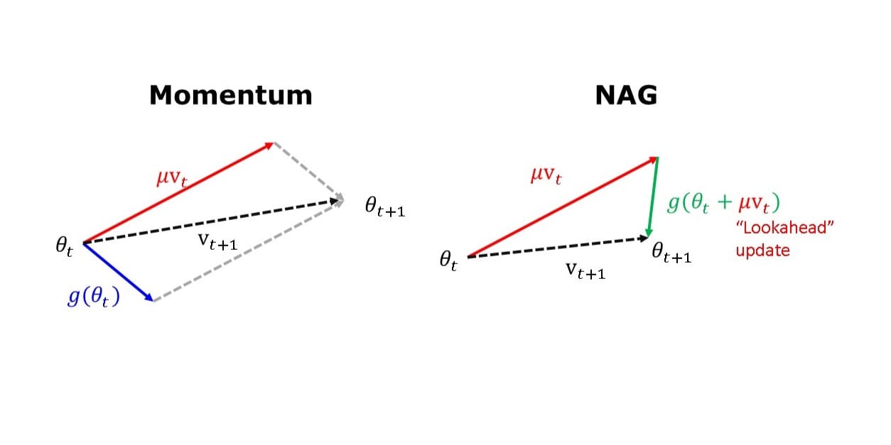
The Nesterov update implements a “lookahead” feature to improve the stability and convergence speed of Momentum for convex functions.
$$ \begin{align*} v_{t+1} &= \red{\mu v_t} - \eta \green{\nabla f(\theta_{t} +} \red{\mu v_t} \green) \\ \theta_{t+1} &= \theta_{t} + v_{t+1} \end{align*} $$
While Momentum uses the current position to update the gradient, NAG performs a partial update of the current position first, knowing that \(\theta_t + \mu v_t \approx θ_{t+1}\).
To implement this as a Python function, I just made the following modification to the “velocity update” in the code I showed before:
# Update velocity

# Momentum
v_t = mu*v_t - eta *grad_f(theta[k-1])

# NAG
v_t = mu*v_t - eta *grad_f(theta[k-1] + mu * v_t)
This partial update helps improve the accuracy of the optimization. In practical terms, it translates into fewer oscillations around a local minimum when compared to Momentum.
The difference is evident in the next figure.
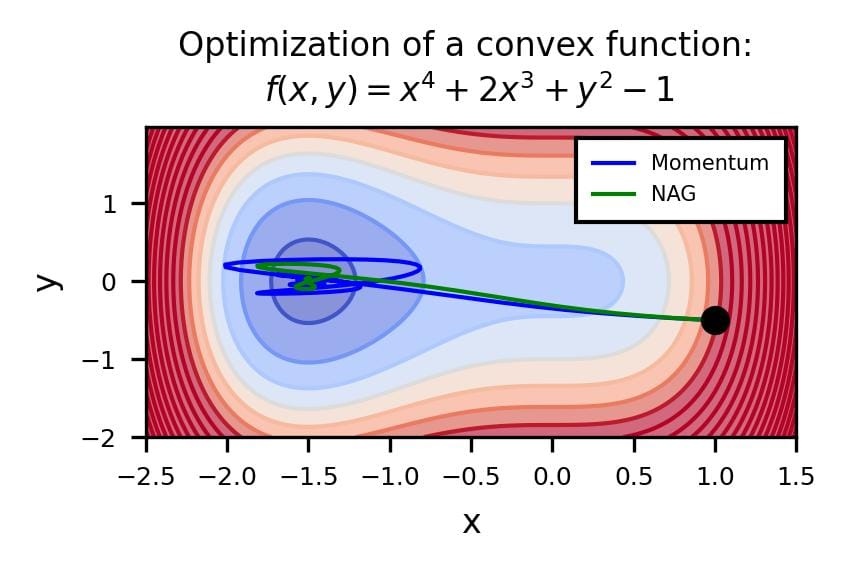
Both optimizers are initialized at the same coordinates, and using the same momentum parameter (0.95, fixed).
The following animation also helps us see the intuition behind scheduling or “annealing” the momentum parameter.
In the beginning, a small amount of momentum can be beneficial to get past the vanishing gradient. When we approach the local minimum, having larger momentum values could dampen out the oscillations we see, improving the convergence speed.
Adaptive methods
The other optimization algorithms shown in the animation above are adaptive methods, which I’ll describe in this section.
Looking at this simple example with a local and a global minimum, Momentum and NAG may seem far superior to the other methods. However, adaptive algorithms are more robust. I’ll show this with a practical example in another article.
Adaptive Gradient Algorithm (AdaGrad)
AdaGrad is a family of subgradient algorithms for stochastic optimization, presented by John Duchi, Elad Hazan and Yoram Singer in 2011.
They proposed to improve gradient-based learning by incorporating the history of the gradients into each new update of the weights.
Instead of biasing the gradient itself, as momentum does, AdaGrad modifies the learning rate dynamically and separately for each parameter of the objective function.
This means we have different learning rates for each model weight. They are adjusted based on the consistency of the gradients.
To do this, the sequence of gradient estimates is stored as follows:
$$ \begin{align*} G_t &= \sum_{\tau = 1}^t g_\tau g_\tau^T \end{align*} $$
If we are optimizing a function with n coordinates or parameters, \(g_t\) will be a vector with n elements, and so will \(G_t\).
Then, the update rule is given by:
$$ \begin{align*} \theta_{t+1} = \theta_t - \frac{\eta}{\sqrt{G_t + \epsilon}} g_t \end{align*} $$
The parameter \(\epsilon\) is used to avoid a division by zero and is usually set to a small value, like 1e-08.
Interestingly, the definition of \(G_t\) is similar to the un-centered (zero-mean) variance of the distribution of gradients.
$$ var = \frac{1}{n}\sum_{i=1}^n (y_i - \bar{y})^2 $$
The variance is a measure of the dispersion energy of a distribution.
Hence, for each parameter \(\theta_i\) , the learning rate is adapted in proportion to the inverse of the gradient's variance for \(\theta_i\).
Considering this, we could say that parameters with more dispersion in their gradient distribution will scale down the learning rate by a larger factor, while those with more consistent gradients (lower variance) will have larger learning rates.
AdaGrad also implements learning rate decay automatically, based on the time (accumulation of previous gradients) and the curvature of the objective function (”areas” with lower gradient variance will be assigned smaller step sizes). This improves the convergence rate of the algorithm.
I’ve implemented AdaGrad as a Python function as follows:
def Adagrad(x_init, y_init, step_size, n_iters):
  eta = step_size
  G_t = 0
  eps = 1e-8

  theta = np.tile([x_init, y_init], (n_iters,1) )
  z = np.tile([f(theta[0])], n_iters )
  for k in range (1, n_iters):
      # Compute gradient
      g_t = grad_f(theta[k-1])

      # Accumulate squared gradients
      G_t += g_t**2

      # Update position
      theta[k] = theta[k-1] - eta * g_t / (np.sqrt(G_t) + eps)
      z[k] = f(theta[k])

  # Store position coordinates
  dataSet = np.stack((theta[:,0], theta[:,1], z), 1)

  return dataSet
One drawback of AdaGrad is that this learning rate decay during training may be too aggressive, causing the learning to stop early when training ANNs. Each parameter update is robust, but the rate at which the changes move toward the optimal point can decrease too much.
Another drawback is that, although the learning rates are self-adjusted during learning, AdaGrad can still be sensitive to the initial conditions. If the gradients are large at the start of the optimization, the learning rates will be low for the rest of the training.
We can see this in the animated figure. AdaGrad breaks off from the symmetry quickly, but the learning is very slow, compared to other algorithms.
To compensate for this, one may need to tune the learning rate to a higher value, which in part defeats the purpose of the self-adjusting characteristic.
Root Mean Square Propagation (RMSprop)
Unpublished method, but mentioned in the slides for lecture 6 of the course Neural Networks for Machine Learning, from Prof. Geoffrey Hinton.
The concept of this algorithm is similar to momentum. It also incorporates the short-term history of the magnitude of the gradients to perform the weights update.
However, similarly to AdaGrad, RMSProp modifies the learning rate and not the gradient.
To do this, the learning rate is divided by a running average of the magnitudes of recent gradients.
First, the algorithm computes a weighted sum of the squared cost values and the previous ones:
$$ \green{\bold v_t} = (1-\green\beta)(dJ)^2 + \green{\beta \bold v_{t-1} }$$
This is like a short-term mean, where the parameter \(\beta\) adjusts how much weight is given to more recent cost values over older ones.
It is analog to the re-written form of momentum that I mentioned before but applied to the squared costs, instead of the gradient.
The next step is dividing the learning rate by the square root of this moving average.
$$ \theta_{t+1} = \theta_{t} - \frac{\eta}{\sqrt{\green{\bold v_t} + \epsilon}} dJ $$
This way, the step size depends on the history of the gradient magnitudes (short-term memory).
Notice that computing the root of a weighted sum (or weighted average) of squared values is equivalent to computing the Root Mean Square (RMS) of those values.
$$ rms = \sqrt{n^{-1}\sum_{i=1}^n y_i^2} $$
The RMS of a signal is a representation of its total energy (as opposed to the variance, which represents its dispersion energy)[1].
Therefore, with RMSProp, the learning rate is modulated according to the total energy of the gradient of the cost function and its previous values. This adjustment is done dynamically and for each direction or component of our loss function (each weight!).
The goal is to reduce the volatility caused by large changes in the gradient by reducing the step size in those cases.
This also helps with vanishing gradient problems because when there’s a trend of very small gradients we take larger steps.
This is how I coded it as a Python function:
def RMSProp(x_init, y_init, step_size, n_iters, decay):
  beta = decay # 0.8, 0.9, ..., 0.99
  eta = step_size
  eps = 1e-8
  MSQ = 0

  theta = np.tile([x_init, y_init], (n_iters,1) )
  z = np.tile([f(theta[0])], n_iters )
  for k in range (1, n_iters):
      # Compute gradient
      g_t = grad_f(theta[k-1])

      # Compute the weighted mean of squared values
      MSQ = beta * MSQ + (1 - beta) * g_t**2

      # Update position (divide eta by RMS)
      theta[k] = theta[k-1] - eta * g_t / (np.sqrt(MSQ) + eps)
      z[k] = f(theta[k])

  # Store position coordinates
  dataSet = np.stack((theta[:,0], theta[:,1], z), 1)

  return dataSet
RMSprop is robust to the initial choice of learning rate, and it also implements an automatic learning rate decay. However, since it is based on a short-term history of gradient values, the decay is less aggressive than AdaGrad.

AdaDelta
Proposed by Matthew Zeiler in 2012.
This method was developed to overcome the main limitations of AdaGrad: the continuous decay of the learning rate that causes early stopping and the need to tune the “global” learning rate manually.
To overcome the continuous learning rate decay, the algorithm accumulates the history of past gradients over a window or fixed size.
In practice, this involves dividing the learning rate by the RMS of previous gradients over a window of fixed size, just like RMSprop does:
$$ \theta_{t+1} = \theta_{t} - \frac{\eta}{\green{\text{RMS}[g]_t}} g_t $$
The next modification from AdaGrad is the correction of the units of the optimization updates.
In AdaGrad (and all other optimization algorithms I’ve described so far), the units of the optimization steps don’t match the units of the parameters that we modify to optimize the cost function [9]:
$$ \text{units of } \Delta\theta \propto \text{units of } \frac{\partial{f}}{\partial{x}}\propto \frac{1}{\text{units of } \theta} $$
We know from school that we can’t add apples and oranges. But with these optimization algorithms, it's like we’ve been adding “apples” (current parameter values, \(\theta_t\) and some unknown quantity (the optimization step \(\Delta\theta\) ) that mathematically can be added to them to obtain new apples (the updated parameters, \(\theta_{t+1}\)). It just works, but doesn’t make sense in real life.
Zeiler decided to correct the units, rearranging the update term from Newton’s method and assuming the curvature of the loss function could be approximated by a diagonal Hessian matrix:
$$ \begin{align*} \text{Newton's method: } x_{n+1} &= x_n - \frac{f(x_n)}{f'(x_n)} \\ x_{n+1} &= x_n - \Delta x \\ \Rightarrow \Delta x &\propto H^{-1}g \propto \frac{\frac{\partial{f}}{\partial{x}}}{\frac{\partial^2{f}}{\partial{x}^2}}\end{align*} $$
Comparing this observation with the update rule similar to RMSProp, Zeiler determined the correct form of the update term to preserve the right units.
The intuition is better explained in the original publication but in practice, it resulted in adding the square root of an exponentially-weighted average of the previous update values to the numerator of the update term:
$$ \Delta\theta_t = - \frac{\text{RMS}[\Delta\theta]_{t-1}}{\green{\text{RMS}[g]_t}} g_t $$
This is basically assuming that the loss function is smooth (low curvature) within a small window of size w, so that \(\Delta\theta_t\) can be approximated by the exponential RMS of the previous values.
The algorithm looks like this if we implement it as a Python function:
def AdaDelta(x_init, y_init, step_size, n_iters, decay):

  eta = step_size
  G_t = 0
  eps = 1e-8
  E_gsq = 0
  E_xsq = 0

  theta = np.tile([x_init, y_init], (n_iters,1) )
  z = np.tile([f(theta[0])], n_iters )
  for k in range (1, n_iters):
      g_t = grad_f(theta[k-1])
      E_gsq = decay * E_gsq + (1 - decay) * g_t**2
      delta = - np.sqrt(E_xsq + eps) / np.sqrt(E_gsq + eps) * g_t
      E_xsq = decay * E_xsq + (1 - decay) * delta**2
      theta[k] = theta[k-1] + delta
      z[k] = f(theta[k])

  # Setting up Data Set for Animation
  dataSet = np.stack((theta[:,0], theta[:,1], z), 1)  # Combining our position coordinates

  return dataSet
AdaDelta combines the advantages of the optimization methods it builds upon.
For instance, the short-term memory of previous parameter updates in the numerator is similar to Momentum and has the effect of accelerating the gradient descent.
The denominator provides the per-dimension accuracy of AdaGrad but without the excessive learning rate decay (just like RMSProp).
Additionally, AdaDelta is more robust to sudden gradient changes, and it is robust to the choice of initial learning rate (see a practical example in the last section of this article).
Adam (Adaptive Momentum)
This is one of the most popular algorithms today.
It was introduced by Diederik P. Kingma and Jimmy Lei Ba in 2014, and has become very popular because of its computational efficiency and because it works very well for problems with large amounts of data and parameters.
Adam is like a combination of Momentum and RMSprop because it dynamically changes both the gradient of the loss function and the learning rates used to scale such gradient to update the weights.
To do this, the algorithm includes the computation of two terms that will be familiar from previous sections of this article.
First, there’s a term from momentum, an exponentially weighted sum of the previous gradients of the cost function (this is like a weighted variance):
$$ \blue{\bold m} = (1-\blue {\beta_1})(dJ) + \blue {\beta_1} \blue{\bold m_{t-1}} $$
Then, there’s a term from RMSprop, an exponentially weighted moving average of the squared gradients.
$$ \green{ \bold v} = (1-\green{\beta_2})(dJ)^2 + \green{\beta_2} \green{\bold v_{t-1}} $$
Combining both terms with the SGD algorithm, the information from past gradients is included in the update step. Their total energy over a short window (RMS) is used to scale the learning rate, and their dispersion (variance) helps adjust the current gradient value used for updating the weights.
$$ \theta_{t+1} = \theta_{t} - \frac{\eta}{\sqrt{\green {\tilde {\bold v}} + \epsilon}} \blue{\tilde {\bold m}} $$
The values with tilde (~) correspond to bias correction terms that are introduced to reduce the contribution from the initial values of m and v as learning progresses:
$$ \blue{\tilde{ {\bold m}}} = \frac{\blue{ \bold m}}{1 - \blue{\beta_1}^t} $$
$$ \green {\tilde{ {\bold v}}} = \frac{\green{ \bold v}}{1 - \green {\beta_2}^t} $$
t = current training epoch.
Unlike AdaDelta, Adam does require tuning of some hyperparameters, but they are easy to interpret.
The terms \(\beta_1\) and \(\beta_2\) are the decay rates of the exponential moving averages of the gradients and the squared gradients, respectively.
Larger values will assign more weight to the previous gradients, giving a smoother behavior, and less reactive to recent changes. Values closer to zero give more weight to recent changes in the gradients. Typical values are \(\beta_1 = 0.9\) and \(\beta_2 = 0.999\).
\(\epsilon\) is, like in all previous cases, a constant added to avoid division by zero, usually set to 1e-8.
Despite having a bunch of additional terms, and significant advantages, Adam is easy to implement:
def Adam(x_init, y_init, step_size, n_iters,
         beta_1 = 0.9, beta_2 = 0.999):

  eps = 1e-8
  eta = step_size

  # Initialize vectors
  m_t = np.array([0,0])
  v_t = np.array([0,0])
  theta = np.tile([x_init, y_init], (n_iters,1) )
  z = np.tile([f(theta[0])], n_iters )

  for k in range (1, n_iters):
      # Compute gradient
      g_t = grad_f(theta[k-1])

      # Compute "momentum-like" term (weighted average)
      m_t = beta_1 * m_t + (1 - beta_1)*g_t

      # Compute the mean of squared gradient values
      v_t = beta_2 * v_t + (1 - beta_2)*g_t**2

      # Initialization bias correction terms
      m_t_hat = m_t/(1 - beta_1**k)
      v_t_hat = v_t/(1 - beta_2**k)

      # Update position with adjusted gradient and lr
      theta[k] = theta[k-1] - eta * m_t_hat/(np.sqrt(v_t_hat)+ eps)
      z[k] = f(theta[k])

  # Store position coordinates
  dataSet = np.stack((theta[:,0], theta[:,1], z), 1)

  return dataSet
Interestingly, the authors of the paper point out that the term \(\frac{\blue{\tilde {\bold m}}}{\sqrt{\green {\tilde {\bold v}}}}\) resembles the definition of the Signal-to-Noise Ratio (SNR):
$$ SNR = \frac{\text{mean}}{\sqrt \text{ variance}}= \frac{\mu}{\sigma} $$
Then, we could say that for smaller SNR values, the parameter updates will be close to zero. This means that we won’t perform large updates whenever there’s too much uncertainty about whether we are moving in the direction of the true gradient.
Adam and its variants typically outperform the other algorithms when training DL models, especially when there are very noisy and sparse gradients.
Performance for different learning rates
I decided to compare how the different optimizers perform when initialized with different “global” learning rates.
This is a rather simple example, but it gives an idea of how these methods are affected by the choice of learning rate.
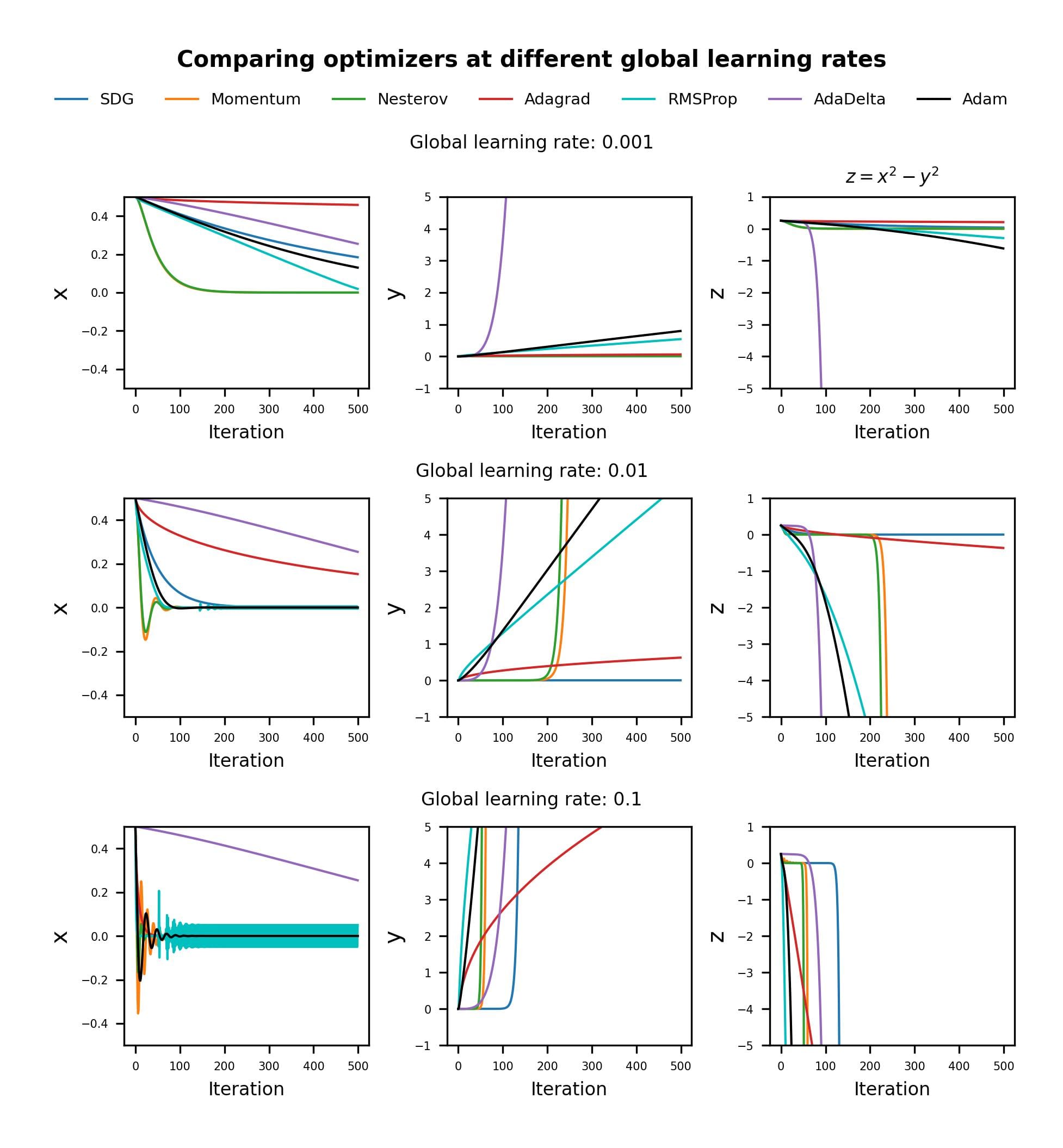
AdaDelta seems remarkably robust to the global learning rate setting, and it “descends” at the same rate for all three cases. We can also see how AdaGrad requires larger learning rates to achieve a performance comparable to AdaDelta in this case.
For small learning rates, it is clear that Adam and RMSProp are similar, and superior to Momentum and SGD.
However, for larger learning rates, RMSProp shows consistent oscillations around the optimum x value (x = 0), while Adam stabilizes after the initial transient, thanks to the dampening effect of the momentum term in the numerator.
The adaptive algorithms break off the symmetry earlier than SGD and Momentum methods, except for the case with a global learning rate of 0.1 for which Momentum and NAG outperform AdaDelta.
Again, these observations only apply to this particular scenario.
Conclusions
The advantages of these optimization algorithms are not fully evident when we apply them to a simple function, like the saddle point example above.
For other scenarios with small-scale models or datasets, even SGD may work better, so it is important to understand where each type of optimizer works best.
When training neural networks, we optimize the Loss function, and we don’t have an exact value of its gradient at any point, just an estimation of it. This is why methods like Adam and AdaDelta, which are robust to noise and sparsity in the gradients have been used widely in the Data Science community.
Also, we can deal with a large amount of model weights, instead of just x and y coordinates. In these scenarios, the ability to obtain per-parameter learning rates is beneficial.
In a future post, I’ll show a more realistic comparison of these methods in another article, using an artificial neural network.
Further reading
- DL Notes: Gradient Descent
- DL Notes: Feed Forwards Artificial Neural Networks
- Creating a Gradient Descent Animation in Python (Towards Data Science)
References
All figures, unless otherwise noted are created by me.
[1] Online course A Deep Understanding of Deep Learning, by Mike X Cohen (sincxpress.com)
[2] Standford Online: CS231 Convolutional Neural Networks for Visual Recognition
[3] Goh. "Why Momentum Really Works", Distill, 2017. http://doi.org/10.23915/distill.00006
[4] Villalarga, D. “AdaGrad”. Published in Cornell University Computational Optimization Open Textbook - Optimization Wiki.
[5] Bengio, Yoshua. "Practical recommendations for gradient-based training of deep architectures." Neural Networks: Tricks of the Trade: Second Edition. Berlin, Heidelberg: Springer Berlin Heidelberg, 437-478, 2012. Online: arXiv:1206.5533 [cs.LG]
[6] Sutskever, I., Martens, J., Dahl, G. & Hinton, G. “On the importance of initialization and momentum in deep learning”. Proceedings of Machine Learning Research, 28(3):1139-1147, 2013. Available from https://proceedings.mlr.press/v28/sutskever13.html.
[7] Duchi, J., Hazan, E., Singer, Y., “Adaptive Subgradient Methods for Online Learning and Stochastic Optimization**”.** Journal of Machine Learning Research, 12(61):2121−2159, 2011*.* Available from: **https://jmlr.org/papers/v12/duchi11a.html
[8] Jason Brownlee, Gradient Descent With AdaGrad From Scratch. 2021
[9] Zeiler, M. “ADADELTA: AN ADAPTIVE LEARNING RATE METHOD”, 2012. arXiv:1212.5701v1 [cs.LG]
[10] Kingma, D., Ba, J. “Adam: A Method for Stochastic Optimization”, 2014. arXiv:1412.6980 [cs.LG]