DL Notes: Feedforward Artificial Neural Networks
I share some notes about the basic math behind feed-forward Artificial Neural Networks (ANNs).


Recently, I decided to learn formally about Machine Learning, and in particular, Artificial Neural Networks. I’ve always been curious about them, but now I need to have a more complete understanding of them to complete some projects in my job, and for some personal projects I want to make.
Today, I will share some notes about the basic math behind Artificial Neural Networks (ANNs). I’ll use them for myself, but also to refer to anyone who asks what the heck am I doing as a side project and why it works.
This is just a high-level overview. A much more in-depth and hands-on explanation of this topic has already been published by Callum Bruce. You should definitely check it out. Also, the math is much clearer in the post published by Jeremy Jordan.
Why
We use the computing power of ANNs to determine relationships across variables when they are too complex for us humans to understand analytically.
To illustrate this, let’s look at the figure below.
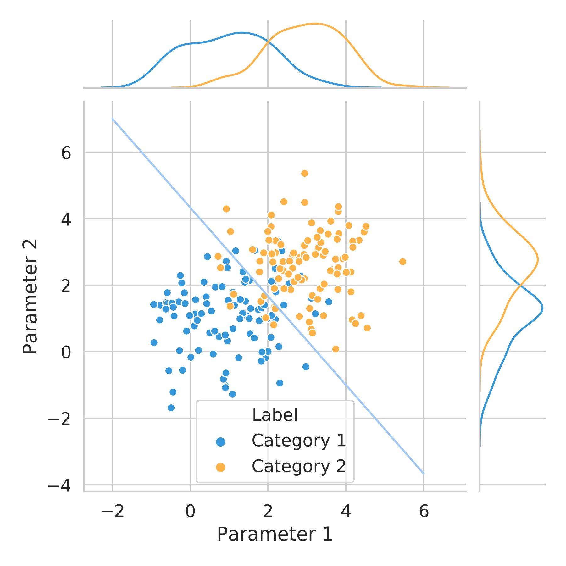
If we wanted to define a criterion to separate the data belonging to each category based on the two parameters available, we could try to accomplish that by drawing a diagonal line like the one depicted in blue.
This line separates the 2-parameter space into two regions. This way, the probability that a variable belongs to Category 1 is high on one side of the line and low on the other. The opposite is true for Category 2.
Notice that the separation isn't perfect, as some points belonging to Category 1 are placed on the side of the line where the majority of points for Category 2 are, and vice-versa. This is why we talk about probability and not certainty.
However, if we need to consider more complex relationships things get difficult for us even to visualize them. If we added a third parameter, we’d get a 3-parameter space, and it would look like the next figure.
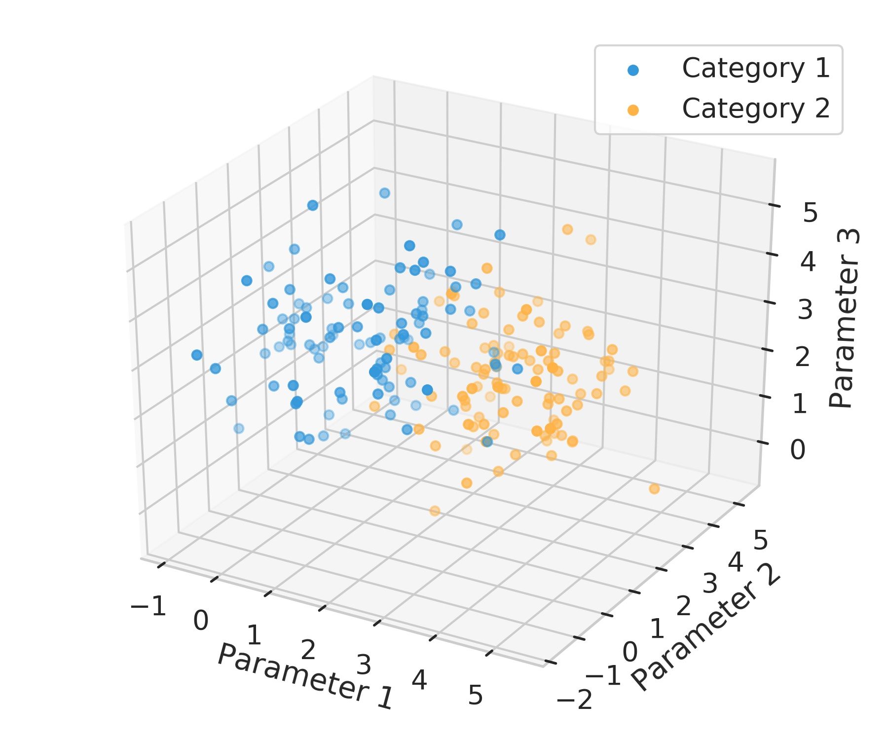
Here, instead of a line to separate the 2D space into two regions, we’d be talking about a surface, known as a hyperplane.
Now, there are problems in many fields that require us to consider N parameters. As the number of parameters grows the more complicated is the relationship between them. We start dealing with high-dimensional spaces.
Neural networks allow us to solve complex problems like this one by performing many simultaneous operations and then repeating them sequentially.
In this case, we are talking about a Classification problem to illustrate the need for computational approaches, but Machine Learning can be used to solve Regression, Clustering, and Dimensionality Reduction problems. ANNs are just one of the many tools available for doing this.
ANNs are interesting because they are universal function approximators, meaning that, provided with sufficient data and trained for enough time, they can approximate any non-linear function. This is very useful in applications when we don’t know the underlying function beforehand.
Of course, there are many different types of ANNs, but I’ll describe here the so-called Feedforward neural networks or Perceptrons.
They were introduced in 1958 [3] , but the advent of higher-performance computing has been critical for their increased popularity in recent years.
These are the most common type of ANNs, and, as their name implies, they are based on the Feedforward process that we will see and are commonly “trained” using an algorithm called backpropagation.
Feedforward
This process is used to feed information through the layers of an ANN. It’s not the only type of algorithm, but it is widely used and the simplest one.
To understand it, let’s look at the following schematic representation of an ANN.
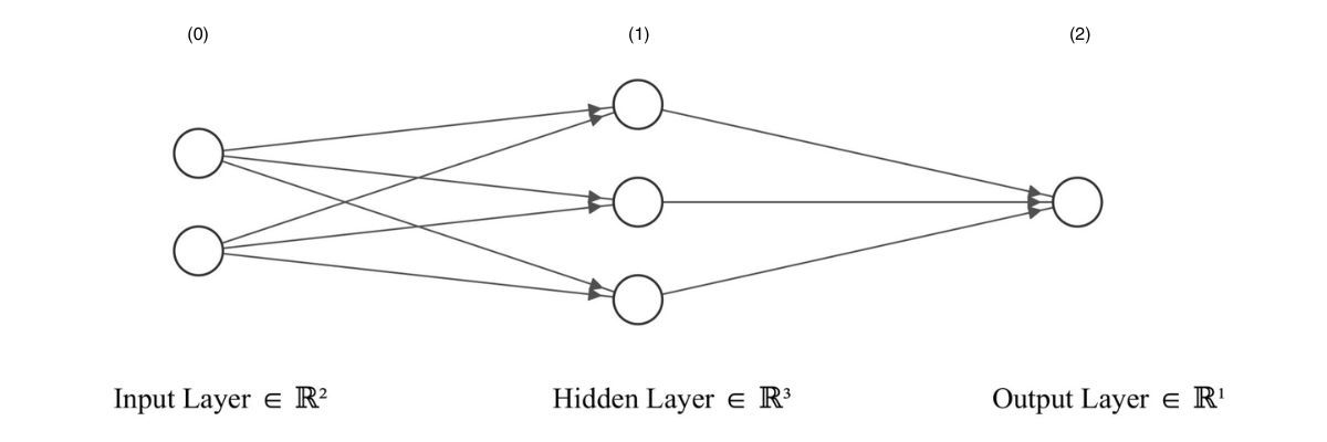
Layers 0 and 2 are called the input and output layers respectively. Any layer between the input and output layer is known as a hidden layer. In this example, we have one hidden layer (layer 1).
How does the information is processed from input to output? Here is when Feedforward comes in.
Each “node” within layer \(l\) performs a weighted sum of the \(m\) outputs of the nodes in the previous layer \(l-1\) that are connected to it, adding an independent bias term. This is basically a linear relationship \(z = x\omega + b\).
Notice that the line separating the 2-parameter space I showed before does not pass through the origin. It is only possible to draw a line like that by adding an “intercept” term, which in this case is the bias term.
The result from this linear operation is passed as an argument to a non-linear function (the so-called activation function), which produces the output from that particular node.
This can be expressed as follows for a single node of layer \(l\) :
$$ y^{l}= \sigma^{l}(x_0^{l}\omega_0^{l} + \sum_{i = 1}^{m} x_i^{l} \omega_i^{l}) \newline y^{l} = \sigma^{l}(b^{l} + \bold{x}^T\bold{w}) \newline y^{l} = \sigma^{l}(\bold{x}^T\bold{w}) $$
Where:
\(\sigma\) = non-linear activation function
\(\omega\) = perceptron model weights (subindex 0 associated with bias term)
\(x\) = inputs (\(x_0\) is shown for formality, but it really is simply equal to 1)
\(b\) = bias term
\(x^{l} = y^{l-1}\)
The subscript \(i\) indicates the \(i^{th}\) element being passed to the node.
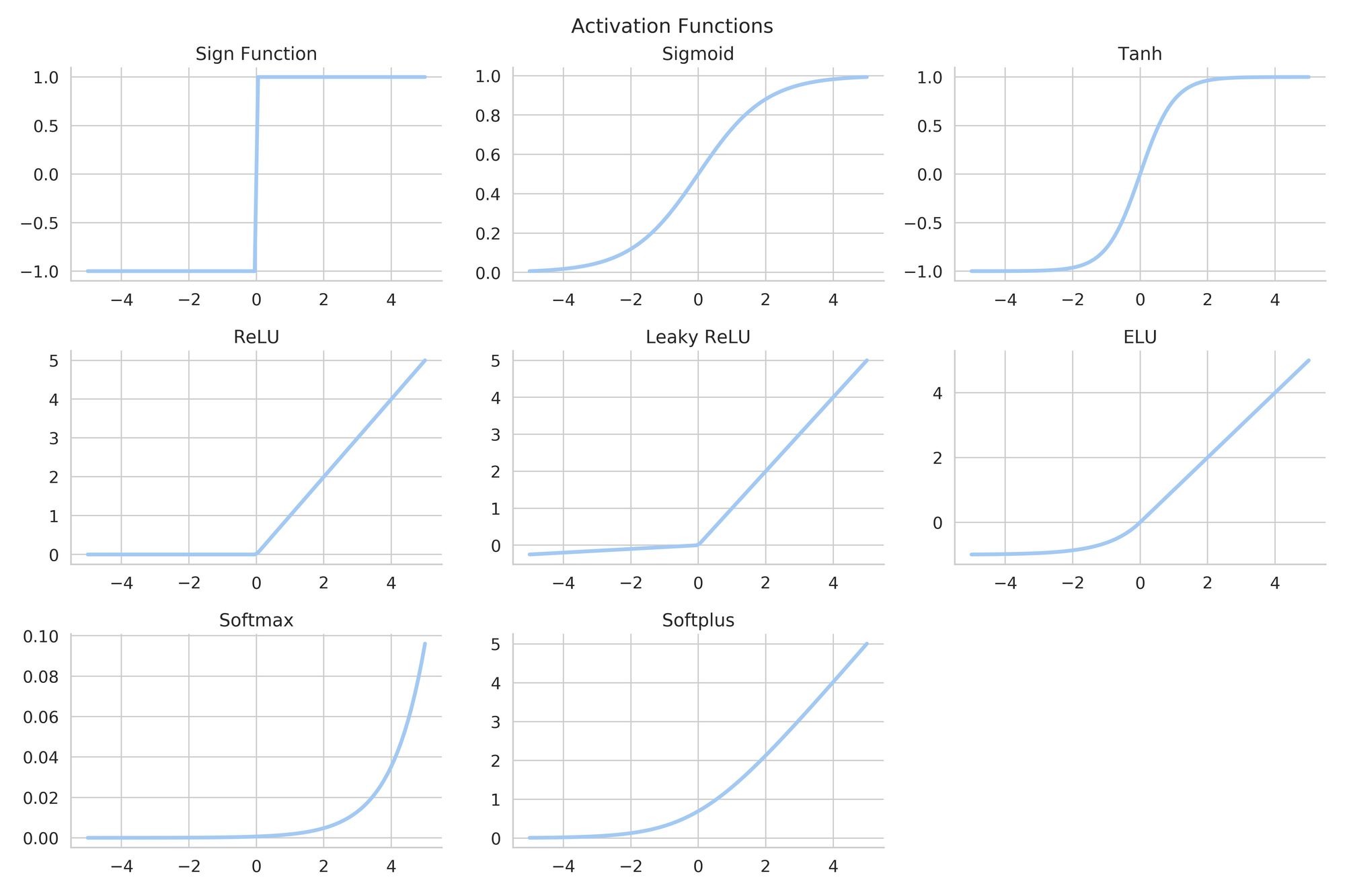
The activation function has the purpose of scaling the output from the weighted average.
There are many types of activation functions, and each one has special characteristics.
They are selected depending on the goal of the layer or the ANN as a whole.
Consider the Classification problem we discussed earlier. If we were to solve it using an ANN, we could use a Sigmoid or a Tanh as an activation function. By mapping the results from the linear operations to a range of values between 0 and 1, we can basically get the probability that a certain sample belongs to Category 1 or Category 2.
Notice that \(\sigma\) is not necessarily the same for the different layers.
This operation is repeated on each node of each layer until the final result is obtained. The input data is “fed” forward.
The whole thing can be expressed in matrix form for computational efficiency.
For example, let’s see what the expression would be like if we wanted to compute all the outputs from the hidden layer of the example ANN we saw before. In matrix form, it would look like this:
\[\begin{bmatrix} y_{0}^{(1)} \\ y_{1}^{(1)} \\ y_{2}^{(1)} \end{bmatrix}=\sigma\left(\begin{bmatrix} w_{0,0} & w_{0,1} & w_{0,2} \\ w_{1,0} & w_{1,1} & w_{1,2} \\ w_{2,0} & w_{2,1} & w_{2,2} \\ \end{bmatrix} \begin{bmatrix} x_{0}^{(1)} \\ x_{1}^{(1)} \\ x_{2}^{(1)} \end{bmatrix}+ \begin{bmatrix} b_{0}^{(1)} \\ b_{1}^{(1)} \\ b_{2}^{(1)} \end{bmatrix} \right) \]
\[\boldsymbol{Y}^{(1)} = \sigma^{(1)}(\bold{W}^{(1)}\boldsymbol{X}^{(1)} + \boldsymbol{b}^{(1)}) \]
\[\boldsymbol{X}^{(2)} = \boldsymbol{Y}^{(1)} \]
As you can see, the core of the feedforward algorithm is reduced to matrix multiplications. And the output from one layer becomes the input for the next one.
Different notations
It might be confusing to find different notations for the abbreviated form of the equation for the activation of a single node:
\[y = \sigma(\bold{wx} + b) \space\space\space\space \rightarrow \space\space\space\space y= \sigma(\bold{x}^T\bold{w}) \]
The two expressions are equivalent. They are used depending on how \(\bold{x}\) and \(\bold{w}\) are represented. From linear algebra, you might recall that, if \(a\) and \(b\) are column vectors,
\[ a\cdot b = b^T a\]
You can also find \(\bold{w}^T\bold{x}\) instead of \(\bold{x}^T\bold{w}\), the former just assumes both \(\bold{w}\) and \(\bold{x}\) are column vectors.
When the bias term is not explicitly shown, it is included in the weights vector, with the corresponding x value equal to 1.
Also, I’ve seen in the literature many authors call the output of the activation function \(a\) (as in “activation”) instead of \(y\), as I’ve done here.
So we've covered the most basic step used for training an ANN. It is important to note that ANNs are not necessarily the best option for solving classification problems. For example, you could look at decision trees or k-means clustering, but I hope the example was useful to show the concepts.
ANNs provide useful data manipulation only after the weights of the net have been correctly adjusted. This is a drastic difference with respect to conventional information processing techniques, where we have step-by-step procedures that can give us a solution. For this reason, we often hear about "training" a neural network. In practice, that simply means adjusting the value of the weights, based on existing data.
From a Digital Signal Processing point of view, you could think about the feed-forward process at the single node level as a convolution of the inputs. Each node multiplies the inputs it receives to correlate them with the set of weights associated with it. A higher correlation will pass a higher value to the activation function. It’s like each node is looking for a pattern in the inputs it receives, and the activation of the node will tell the fractional probability that the pattern exists [2].
Now it's time to look at funkier stuff - backpropagation and gradient descent- but I’ll leave that for the next post. They are the main mechanisms used for "training" an Artificial Neural Network.
References
[1] Online course A deep understanding of Deep Learning, by Mike X Cohen.
[2] S. W. Smith, The Scientist and Engineer's Guide to Digital Signal Processing, Second Edition. 1999