Replacing MATLAB with Python - Part 2: Formatting subplots and indexing data
I used Python to complete the first part of the task from my previous post in the series. I learned about formatting plots and indexing Pandas dataframes.


A couple of weeks ago, I published the second entry of the Replacing MATLAB with Python series I started in August. I am sharing examples of how to do that, with some comments about the problems I find while learning Python.
In the previous post of the series, I didn’t really share any Python code, though. It was an example of how I would use MATLAB to get information from raw data collected from a race car’s CAN bus.
In this entry, I’m using Python to do the first part of the task: visualize the signals we have by creating a figure with subplots, filter the raw acceleration data, compute the vehicle speed for the two drivers, and compare it. It took me more than twice the time to do it in Python than it did with MATLAB. That’s mainly because I have been using MATLAB for many years now, and I am just getting used to Python. Especially when formatting plots, there are several things to handle differently from Matlab, or even from one Python library to another.
As always, bear in mind that this is not intended to be a Python course, but rather a series of practical examples.
Alright, to the code!
Importing the data
I’m following the same workflow that I used for the MATLAB version of this, where I also provided more context on what we have. Short story, we want to compare the performance of two drivers, and we have the car data for each one in separate CSV files.


This is the code I wrote to start with. We’ve already seen how to load information from CSV files and use Pandas to handle our data.
When using Python, the first thing we do is import the libraries we are going to use. We don’t necessarily have to put the imports on top of everything, but it’s in general good practice.
#%% Import libraries
import pandas as pd
import numpy as np
import matplotlib.pyplot as plt

#%% Load data from CSV files

df1 = pd.read_csv('driver1.csv')
print(df1.columns)

df2 = pd.read_csv('driver2.csv')
print(df2.columns)

#%% Define constants
gear_ratio = 16     # Transmission gear ratio
r = 0.263           # Wheel radius [m]

>> Index(['Time_s', 'BrakeFront', 'AccX', 'spd_rpmFL', 'spd_rpmFR', 'spd_rpmRL',
       'spd_rpmRR'],
        dtype='object')
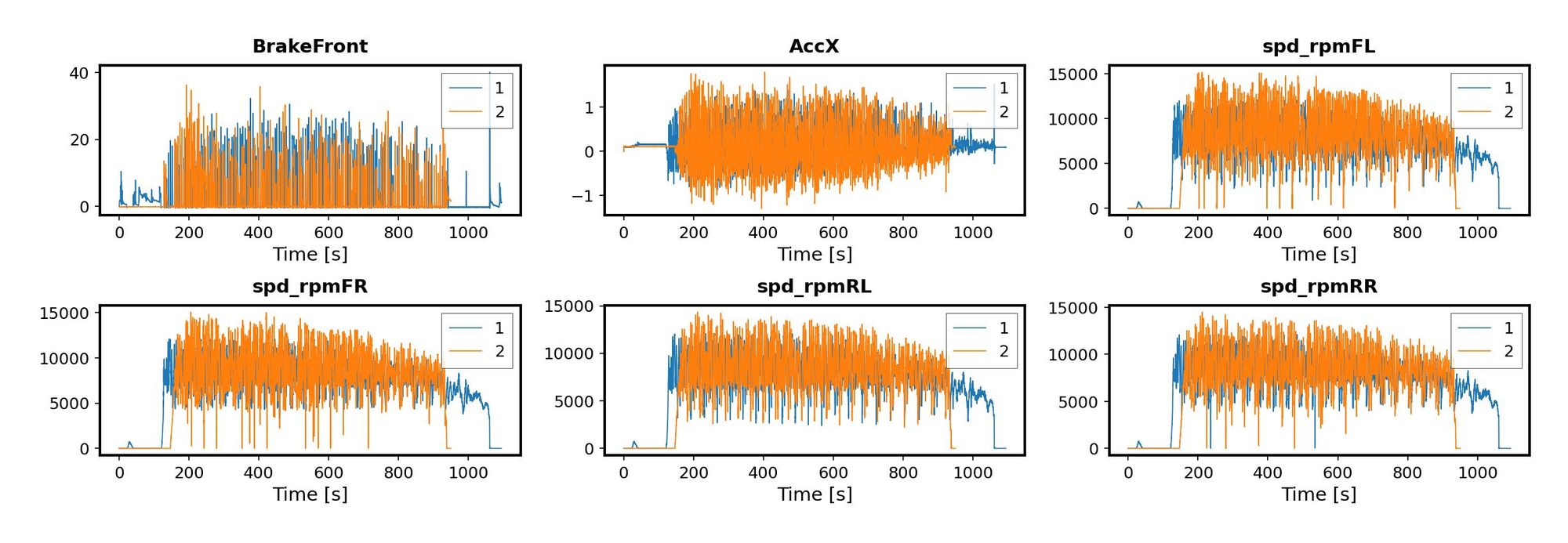
All good! We have a unique time base and 6 signals in each file. But we have to make sure they are consistent and can be used together. This is why the next thing I did in MATLAB was plotting the variables.
When I tried to do the same thing using Python, it took me a while. More than I am comfortable admitting. I was stubbornly trying to get the exact same look I got with the default settings in MATLAB and, obviously, that required a lot of formatting. At some point I got it, but the number of trials with format options was just not worth it. Just look at the plt.rcParams.update call at the bottom of the next code snippet! My advice: if you are replacing MATLAB with Python, don’t try to get exactly the same look on your charts unless there is a real need for that- in my case, there wasn’t.
# If needed, reset plot parameters from any previous plot
# plt.rcParams.update(plt.rcParamsDefault)

fig = plt.figure(figsize = (1200/300, 600/300), dpi = 300)

c = 1 # subplot counter
for col in df1.columns[1:]:
    ax = plt.subplot(3, 3, c)
    ax.plot(df1['Time_s'], df1[col], label = '1', linewidth = 0.2)
    ax.plot(df2['Time_s'], df2[col], label = '2', linewidth = 0.2)
    leg = ax.legend(edgecolor = 'black',
                    borderpad=.5, borderaxespad = .5,
                    fontsize = 3, fancybox = False,
                    loc = 'upper right')
    plt.xlabel('Time [s]', fontsize = 3.5)
    plt.title( col, fontweight="bold", y = 1.05, fontsize = 3.5)
    leg.get_frame().set_linewidth(.1)
    c = c + 1

plt.rcParams.update({'axes.grid': False,
                    'xtick.labelsize': 3,
                    'ytick.labelsize': 3,
                    'axes.labelpad': 1.0,
                    'axes.labelsize': 3.5,
                    'axes.linewidth': 0.5,
                    'ytick.major.pad': 1,
                    'ytick.minor.left': False,
                    'xtick.minor.bottom': False,
                    'ytick.major.size': 1,
                    'ytick.major.width': .2,
                    'xtick.major.pad': 1,
                    'xtick.major.size': 1,
                    'xtick.major.width': .2})

fig.tight_layout()

fig.subplots_adjust(
    top=0.92,
    bottom=0.1,
    left=0.05,
    right=0.98,
    hspace=0.6,
    wspace=0.2
)

fig
Some of the useful resources I found online to learn about formatting are: first of all, Matplotlib's official documentation. Second, the countless number of sites with Python tutorials online - just googled my questions and found good answers in the first page of results. Third, previously-answered questions on stackoverflow.
Something nice about Python is that we are able to iterate directly through the columns of our dataframe, instead of creating an index and then slicing the dataframe by column position. By doing it this way, I just needed to make a counter to move to the next plot, and the data was selected from the current column. The results are not identical to the ones I got in MATLAB, but that’s OK.
All this additional formatting is needed only if you are using the relatively low-level library Pyplot and you want to get some really specific format. If you loosen the format a bit and open up to other options - like Seaborn for example - you can actually get away with very little code to get some impressive plots. Or, if you need to make interactive plots, you could use Plotly, like I did when visualizing how warped the bed of my 3D printer was. I’ll show another example next, when we compare the speeds of the two drivers.
Fine, we can make plots without stressing too much about the format and live with it.
Let’s move on.
Filtering acceleration data
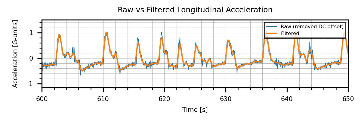
As in the MATLAB example, I used a digital filter to smooth the acceleration signals. I’m filtering only those because they are the only ones containing raw data from sensors. Here’s what the raw acceleration data looks like when compared against the filtered one:
The code I used for doing this is quite simple.
First, I computed the sum of the speeds of the four in-wheel motors. To do this, I needed to select only the columns for those variables, and compute the sum for each row. In MATLAB we can select data from tables using numerical indices and round parenthesis directly, and the result is a table object. With Python, to index a dataframe this way, we need to use the iloc method. This allows you to slice the dataframe using numerical indices. In this case, I selected all the rows, and then the columns from the third one till the end, so the returned object is also a dataframe.
To compute the sum of each row, I used the sum method of dataframes, passing as argument axis = 1 to indicate that I want to sum each row and put the results in a column. For dataframes, rows are axis 0 and columns are axis 1. This is equivalent to MATLAB's concept of rows and columns in tables. So when I sum along axis 1, I add all the column values on each row.
The results are stored in new columns named 'SumSpeeds' in the original dataframes.
df1['SumSpeeds'] = df1.iloc[:,3:].sum(axis=1)
df2['SumSpeeds'] = df2.iloc[:,3:].sum(axis=1)Cool! Next, I removed the DC offsets from the acceleration signals. I selected only the rows in which the sum of the speeds was zero and computed the median of the acceleration values. Then I subtracted this non-zero offset from the acceleration signals. This is how I did that:
df1['AccX_NoOffs'] = df1['AccX'] - df1[df1['SumSpeeds'] == 0]['AccX'].median()
df2['AccX_NoOffs'] = df2['AccX'] - df2[df2['SumSpeeds'] == 0]['AccX'].median()In this case, I sliced the dataframe using a different approach. I compared the 'SumSpeeds' column with zero, creating a series object with logical statements (True/False). This is equivalent to doing myseries = df_A['SumSpeeds'] == 0. Then, I sliced the original dataframes using that series as an index. This returned a new dataframe containing all the rows in which the condition is met, and all the columns, as in df_B = df_A[myseries]. Finally, I selected the 'AccX' column from the resulting dataframe and computed the median from it. It would have looked like DC_offset = df_B['AccX'].median(). And this is what I subtracted from the original signals.
The last part was filtering the corrected signals and finally making the figure I previously showed, comparing the raw and filtered signals:
from scipy.signal import savgol_filter

df1.AccX = savgol_filter(df1.AccX_NoOffs, 101, 3)
df2.AccX = savgol_filter(df2.AccX_NoOffs, 101, 3)

# reset figure parameters if previously changed
#plt.rcParams.update(plt.rcParamsDefault)

# Compare raw acceleration vs filtered
fig = plt.figure(figsize = (1200/300, 400/300), dpi=300)
plt.plot(df1.Time_s, df1.AccX_NoOffs, label = 'Raw (removed DC offset)', linewidth = .5)
plt.plot(df1.Time_s, df1.AccX, label = 'Filtered', linewidth = 1)
plt.xlabel('Time [s]')
plt.ylabel("Acceleration [G-units]")
plt.xlim(600, 650)

leg = plt.legend(fancybox = False,
                edgecolor = 'inherit', fontsize = 4,
                loc = 'upper right')


plt.title('Raw vs Filtered Longitudinal Acceleration')

plt.rcParams.update({'font.size': 5,
                    'axes.grid': True,
                    'axes.grid.which': 'both',
                    'xtick.minor.visible': True,
                    'ytick.minor.visible': True,
                    'grid.linewidth': 0.2,
                    'lines.linewidth': 0.2})


# Display figure
plt.tight_layout()
figI implemented the same type of filter I used in MATLAB, I just needed an additional library import. However, the input arguments for the Python version savgol_filter(data_array, window_size, poly_order) are swapped with respect to MATLAB’s (recall I used sgolayfilt(data_array, poly_order, window_size) in the previous post). We can spot this kind of thing by looking at the documentation. Always read the documentation! With Python, you can access it quickly by typing print(<library,object or function>.__doc___) or simply help(<library,object or function>) .
Unfortunately, the official documentation for many Python functions is not as detailed as the MATLAB counterpart. For instance, compare the MATLAB and Python (Scypi) official documentation for the filter we used. The former is much clearer. This can be a big thing for many people wanting to learn Python coming from MATLAB, but there is a way to go around it! There are a lot more tutorials online about Python than there are for MATLAB. You just have to embrace the power of googling, and lose the fear of sites like stackoverflow. For example, I found this great article about the filter we are using. Additionally, the best thing to do is check some Signal Processing book to learn more about digital filters.
Ok! I am deviating from the point of this article. Going back to the code examples.
Finding the vehicle speed: indexing dataframes
As I mentioned in the MATLAB example, we can estimate the vehicle speed using the information from the speeds of the four in-wheel motors. We just need to treat differently the cases in which the vehicle was accelerating and those in which it was braking. To do this, we'll need to index (slice) the dataframe based in conditions similar to what I did with the raw acceleration data when computing the DC offset. See how I did it in the code below:
import timeit

%%timeit

df1['Vehicle Speed'] = 0
df2['Vehicle Speed'] = 0

# Estimated vehicle speeds when braking (AccX < = 0)
df1.loc[df1['AccX'] <= 0, 'Vehicle Speed'] =  df1.loc[df1['AccX'] <= 0,
                                            ('spd_rpmFL','spd_rpmFR','spd_rpmRL','spd_rpmRR')].max(axis=1)*np.pi/30*r/gear_ratio*3.6
df2.loc[df2['AccX'] <= 0, 'Vehicle Speed'] =  df2.loc[df2['AccX'] <= 0,
                                            ('spd_rpmFL','spd_rpmFR','spd_rpmRL','spd_rpmRR')].max(axis=1)*np.pi/30*r/gear_ratio*3.6

# Estimated vehicle speeds when accelerating (AccX > 0)
df1.loc[df1['AccX'] > 0, 'Vehicle Speed'] =  df1.loc[df1['AccX'] > 0,
                                            ('spd_rpmFL','spd_rpmFR','spd_rpmRL','spd_rpmRR')].min(axis=1)*np.pi/30*r/gear_ratio*3.6
df2.loc[df2['AccX'] > 0, 'Vehicle Speed'] =  df2.loc[df2['AccX'] > 0,
                                            ('spd_rpmFL','spd_rpmFR','spd_rpmRL','spd_rpmRR')].min(axis=1)*np.pi/30*r/gear_ratio*3.6

# Output 62.2 ms ± 3.78 ms per loop (mean ± std. dev. of 7 runs, 10 loops each)
That was very quick. As you can see, if you get used to indexing MATLAB tables, the switch to Pandas dataframes is a lot easier. The syntax (or rather, the logic) is very similar - though it is not exactly the same.
Now, we can just compare the speeds. First, I computed the start and end times for both drivers. This is not precise, I just defined a speed threshold of 20 km/h and found the instants when the car was slower and faster than that. Again, dataframe slicing is very helpful for this:
# Find index of first instant at which speed is greater than 20 km/h
index_start1 = df1[df1['Vehicle Speed']>20].index[0]
index_start2 = df2[df2['Vehicle Speed']>20].index[0]
time_start1 = df1['Time_s'][index_start1]
time_start2 = df2['Time_s'][index_start2]

# Find index of last instant at which speed is greater than 20 km/h
index_end1 = df1[df1['Vehicle Speed']>20].index[-1]
index_end2 = df2[df2['Vehicle Speed']>20].index[-1]
time_end1 = df1['Time_s'][index_end1]
time_end2 = df2['Time_s'][index_end2]

# Compute elapsed times
t_elap_1 = time_end1 - time_start1
t_elap_2 = time_end2 - time_start2
Next, I made a comparative plot (subplots again). This time with a different approach, though:
# %% Compare the speeds of the two drivers
from plotly.subplots import make_subplots
import plotly.graph_objects as go


# Create figure with subplots and add titles
fig = make_subplots(
    rows=2,
    cols=1,
    shared_xaxes=True,
    shared_yaxes=False,
    subplot_titles=((f"Driver 1 approximate time : {t_elap_1:.1f} seconds<br>"
                     f"Max. speed: {df1['Vehicle Speed'].max():.1f} km/h, "
                     f"mean speed: {df1['Vehicle Speed'].mean():.1f} km/h"),
                    (f"Driver 2 approximate time : {t_elap_2:.1f} seconds<br>"
                    f"Max. Speed: {df2['Vehicle Speed'].max():.1f} km/h, "
                    f"mean speed: {df2['Vehicle Speed'].mean():.1f} km/h")
))

# Plot data for the first driver
fig.add_trace(
    go.Line(y=df1['Vehicle Speed'] ,x=df1.Time_s,name = 'Driver 1'),
    row = 1, col = 1)
# Add vertical lines to mark start and end points
for time in [time_start1, time_end1]:
    fig.add_shape(go.layout.Shape(type = "line",
                                    yref = "y", xref = "x",
                                    x0 = time, y0=0,
                                    x1 = time, y1 = 100),
                                    row=1, col=1)
fig.update_yaxes(title_text="Speed [km/h]", range=[0, 100], row=1, col=1)

# Plot data for the second driver
fig.add_trace(
    go.Line(y=df2['Vehicle Speed'] ,x=df1.Time_s,name = 'Driver 2'),
    row = 2, col = 1)
# Add vertical lines to mark start and end points
for time in [time_start2, time_end2]:
    fig.add_shape(go.layout.Shape(type = "line",
                                    yref = "y", xref = "x",
                                    x0 = time, y0=0,
                                    x1 = time, y1 = 100),
                                    row=2, col=1)
fig.update_yaxes(title_text="Speed [km/h]", range=[0, 100], row=2, col=1)

fig.update_layout(title = {
                            'text': '<b>Driver time comparison</b>',
                            'xanchor' : 'center',
                            'x' : 0.5, 'y': .95, 'font_size' : 20
                            },
                showlegend=False)

fig
Notice that I used Plotly instead of Pyplot. Confusing names, right? Pyplot is the “vanilla” one that comes with Matplotlib. It is easier to learn when starting with Python from a Matlab background and is used a lot for scientific and engineering publication-grade figures. But Plotly offers the possibility to make interactive plots with a little coding, which is awesome. Just look at the results:
Wrapping up
We completed the first part of the task, obtaining the same results as the Matlab example - fortunately! otherwise, there would be a great error somewhere.
When writing this, I think I spent 80% of my time figuring out how to make the plots look like I wanted. The rest was not really that hard. This is not surprising, since Python has gained popularity precisely for being easy to learn. It is easy, as long as you use it as it is intended to. The best way to achieve this is to follow a set of guidelines for coding style, which are known as the “Pythonic” way. I will try to learn this and apply it to my code as I go. I think it makes you think more in terms of code efficiency and make better use of the language.
I hope these code examples were useful for you. In the next post, I will complete the second part of the task, using histograms and statistics to analyze the vehicle speeds and the braking performance of the two drivers.
In the meantime, I hope you have a wonderful day!